

402
7.2. QUALITATIVE BEHAVIOR OF SOLUTIONS TO DES
1
2
3
-2
-1
1
2
3
t
y
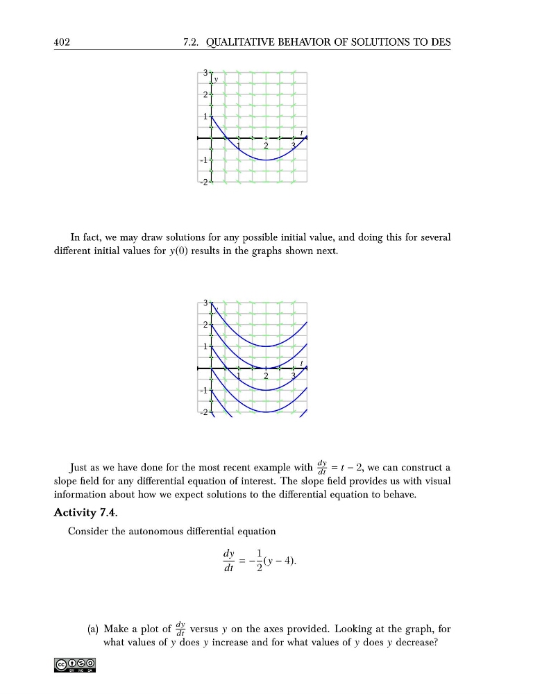
In fact, we may draw solutions for any possible initial value, and doing this for several
different initial values for y(0) results in the graphs shown next.
1
2
3
-2
-1
1
2
3
t
y
Just as we have done for the most recent example with
dy
dt = t − 2, we can construct a
slope field for any differential equation of interest. The slope field provides us with visual
information about how we expect solutions to the differential equation to behave.
Activity 7.4.
Consider the autonomous differential equation
dy
dt
= −
1
2
(y − 4).
(a) Make a plot of
dy
dt versus y on the axes provided. Looking at the graph, for
what values of y does y increase and for what values of y does y decrease?
7.2. QUALITATIVE BEHAVIOR OF SOLUTIONS TO DES
1
2
3
-2
-1
1
2
3
t
y
In fact, we may draw solutions for any possible initial value, and doing this for several
different initial values for y(0) results in the graphs shown next.
1
2
3
-2
-1
1
2
3
t
y
Just as we have done for the most recent example with
dy
dt = t − 2, we can construct a
slope field for any differential equation of interest. The slope field provides us with visual
information about how we expect solutions to the differential equation to behave.
Activity 7.4.
Consider the autonomous differential equation
dy
dt
= −
1
2
(y − 4).
(a) Make a plot of
dy
dt versus y on the axes provided. Looking at the graph, for
what values of y does y increase and for what values of y does y decrease?