

7.2. QUALITATIVE BEHAVIOR OF SOLUTIONS TO DES
399
1
2
3
-2
-1
1
2
3
t
y
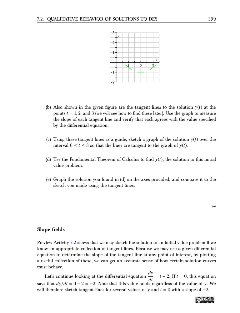
(b) Also shown in the given figure are the tangent lines to the solution y(t) at the
points t = 1, 2, and 3 (we will see how to find these later). Use the graph to measure
the slope of each tangent line and verify that each agrees with the value specified
by the differential equation.
(c) Using these tangent lines as a guide, sketch a graph of the solution y(t) over the
interval 0 ≤ t ≤ 3 so that the lines are tangent to the graph of y(t).
(d) Use the Fundamental Theorem of Calculus to find y(t), the solution to this initial
value problem.
(e) Graph the solution you found in (d) on the axes provided, and compare it to the
sketch you made using the tangent lines.
⊲⊳
Slope fields
Preview Activity 7.2 shows that we may sketch the solution to an initial value problem if we
know an appropriate collection of tangent lines. Because we may use a given differential
equation to determine the slope of the tangent line at any point of interest, by plotting
a useful collection of these, we can get an accurate sense of how certain solution curves
must behave.
Let’s continue looking at the differential equation
dy
dt
= t − 2. If t = 0, this equation
says that dy/dt = 0 − 2 = −2. Note that this value holds regardless of the value of y. We
will therefore sketch tangent lines for several values of y and t = 0 with a slope of −2.
399
1
2
3
-2
-1
1
2
3
t
y
(b) Also shown in the given figure are the tangent lines to the solution y(t) at the
points t = 1, 2, and 3 (we will see how to find these later). Use the graph to measure
the slope of each tangent line and verify that each agrees with the value specified
by the differential equation.
(c) Using these tangent lines as a guide, sketch a graph of the solution y(t) over the
interval 0 ≤ t ≤ 3 so that the lines are tangent to the graph of y(t).
(d) Use the Fundamental Theorem of Calculus to find y(t), the solution to this initial
value problem.
(e) Graph the solution you found in (d) on the axes provided, and compare it to the
sketch you made using the tangent lines.
⊲⊳
Slope fields
Preview Activity 7.2 shows that we may sketch the solution to an initial value problem if we
know an appropriate collection of tangent lines. Because we may use a given differential
equation to determine the slope of the tangent line at any point of interest, by plotting
a useful collection of these, we can get an accurate sense of how certain solution curves
must behave.
Let’s continue looking at the differential equation
dy
dt
= t − 2. If t = 0, this equation
says that dy/dt = 0 − 2 = −2. Note that this value holds regardless of the value of y. We
will therefore sketch tangent lines for several values of y and t = 0 with a slope of −2.