

356
6.3. DENSITY, MASS, AND CENTER OF MASS
If we consider the formula m = d · V , it is reminiscent of two other equations that we
have used frequently in recent work: for a body moving in a fixed direction, distance =
rate · time, and, for a rectangle, its area is given by A = l · w. These formulas hold when
the principal quantities involved, such as the rate the body moves and the height of the
rectangle, are constant. When these quantities are not constant, we have turned to the
definite integral for assistance. The main idea in each situation is that by working with
small slices of the quantity that is varying, we can use a definite integral to add up the
values of small pieces on which the quantity of interest (such as the velocity of a moving
object) are approximately constant.
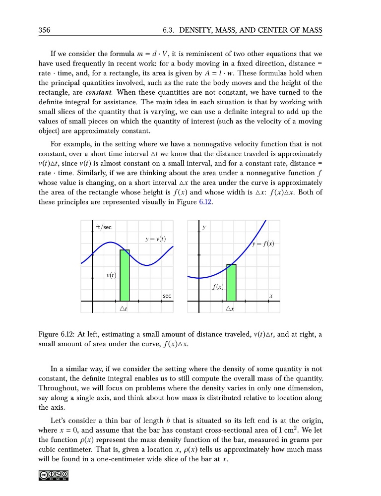
For example, in the setting where we have a nonnegative velocity function that is not
constant, over a short time interval △t we know that the distance traveled is approximately
v(t)△t, since v(t) is almost constant on a small interval, and for a constant rate, distance =
rate · time. Similarly, if we are thinking about the area under a nonnegative function f
whose value is changing, on a short interval △x the area under the curve is approximately
the area of the rectangle whose height is f (x) and whose width is △x: f (x)△x. Both of
these principles are represented visually in Figure 6.12.
ft/sec
sec
y = v(t)
v(t)
△t
y
x
y = f (x)
f (x)
△x
Figure 6.12: At left, estimating a small amount of distance traveled, v(t)△t, and at right, a
small amount of area under the curve, f (x)△x.
In a similar way, if we consider the setting where the density of some quantity is not
constant, the definite integral enables us to still compute the overall mass of the quantity.
Throughout, we will focus on problems where the density varies in only one dimension,
say along a single axis, and think about how mass is distributed relative to location along
the axis.
Let’s consider a thin bar of length b that is situated so its left end is at the origin,
where x = 0, and assume that the bar has constant cross-sectional area of 1 cm 2 . We let
the function ρ(x) represent the mass density function of the bar, measured in grams per
cubic centimeter. That is, given a location x, ρ(x) tells us approximately how much mass
will be found in a one-centimeter wide slice of the bar at x.
6.3. DENSITY, MASS, AND CENTER OF MASS
If we consider the formula m = d · V , it is reminiscent of two other equations that we
have used frequently in recent work: for a body moving in a fixed direction, distance =
rate · time, and, for a rectangle, its area is given by A = l · w. These formulas hold when
the principal quantities involved, such as the rate the body moves and the height of the
rectangle, are constant. When these quantities are not constant, we have turned to the
definite integral for assistance. The main idea in each situation is that by working with
small slices of the quantity that is varying, we can use a definite integral to add up the
values of small pieces on which the quantity of interest (such as the velocity of a moving
object) are approximately constant.
For example, in the setting where we have a nonnegative velocity function that is not
constant, over a short time interval △t we know that the distance traveled is approximately
v(t)△t, since v(t) is almost constant on a small interval, and for a constant rate, distance =
rate · time. Similarly, if we are thinking about the area under a nonnegative function f
whose value is changing, on a short interval △x the area under the curve is approximately
the area of the rectangle whose height is f (x) and whose width is △x: f (x)△x. Both of
these principles are represented visually in Figure 6.12.
ft/sec
sec
y = v(t)
v(t)
△t
y
x
y = f (x)
f (x)
△x
Figure 6.12: At left, estimating a small amount of distance traveled, v(t)△t, and at right, a
small amount of area under the curve, f (x)△x.
In a similar way, if we consider the setting where the density of some quantity is not
constant, the definite integral enables us to still compute the overall mass of the quantity.
Throughout, we will focus on problems where the density varies in only one dimension,
say along a single axis, and think about how mass is distributed relative to location along
the axis.
Let’s consider a thin bar of length b that is situated so its left end is at the origin,
where x = 0, and assume that the bar has constant cross-sectional area of 1 cm 2 . We let
the function ρ(x) represent the mass density function of the bar, measured in grams per
cubic centimeter. That is, given a location x, ρ(x) tells us approximately how much mass
will be found in a one-centimeter wide slice of the bar at x.