

5.6. NUMERICAL INTEGRATION
327
Table 5.1, but include additional results for S 8 =
2M 4 +T 4
3
and S 16 =
2M 8 +T 8
3
.
1
0
(1 − x 2 ) dx = 0.6 error
2
1
1
x 2 dx = 0.5 error
T 4
0.65625
-0.0104166667
0.5089937642
0.0089937642
M 4 0.671875
0.0052083333 0.4955479365 -0.0044520635
S 8
0.6666666667
0
0.5000298792 0.0000298792
T 8
0.6640625
-0.0026041667 0.5022708502
0.0022708502
M 8 0.66796875
0.0013020833 0.4988674899 -0.0011325101
S 16 0.6666666667
0
0.5000019434
0.0000019434
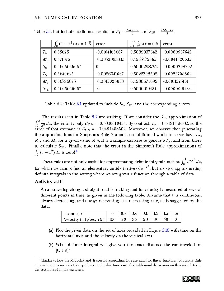
Table 5.2: Table 5.1 updated to include S 8 , S 16 , and the corresponding errors.
The results seen in Table 5.2 are striking. If we consider the S 16 approximation of
2
1
1
x 2 dx, the error is only E S,16 = 0.0000019434. By contrast, L 8 = 0.5491458502, so the
error of that estimate is E L,8 = −0.0491458502. Moreover, we observe that generating
the approximations for Simpson’s Rule is almost no additional work: once we have L n ,
R n , and M n for a given value of n, it is a simple exercise to generate T n , and from there
to calculate S 2n . Finally, note that the error in the Simpson’s Rule approximations of
1
0
(1 − x 2 ) dx is zero! 10
These rules are not only useful for approximating definite integrals such as
1
0
e −x 2 dx,
for which we cannot find an elementary antiderivative of e −x 2 , but also for approximating
definite integrals in the setting where we are given a function through a table of data.
Activity 5.16.
A car traveling along a straight road is braking and its velocity is measured at several
different points in time, as given in the following table. Assume that v is continuous,
always decreasing, and always decreasing at a decreasing rate, as is suggested by the
data.
seconds, t
0
0.3 0.6 0.9 1.2 1.5 1.8
Velocity in ft/sec, v(t) 100 99 96 90 80 50 0
(a) Plot the given data on the set of axes provided in Figure 5.18 with time on the
horizontal axis and the velocity on the vertical axis.
(b) What definite integral will give you the exact distance the car traveled on
[0, 1.8]?
10 Similar to how the Midpoint and Trapezoid approximations are exact for linear functions, Simpson’s Rule
approximations are exact for quadratic and cubic functions. See additional discussion on this issue later in
the section and in the exercises.
327
Table 5.1, but include additional results for S 8 =
2M 4 +T 4
3
and S 16 =
2M 8 +T 8
3
.
1
0
(1 − x 2 ) dx = 0.6 error
2
1
1
x 2 dx = 0.5 error
T 4
0.65625
-0.0104166667
0.5089937642
0.0089937642
M 4 0.671875
0.0052083333 0.4955479365 -0.0044520635
S 8
0.6666666667
0
0.5000298792 0.0000298792
T 8
0.6640625
-0.0026041667 0.5022708502
0.0022708502
M 8 0.66796875
0.0013020833 0.4988674899 -0.0011325101
S 16 0.6666666667
0
0.5000019434
0.0000019434
Table 5.2: Table 5.1 updated to include S 8 , S 16 , and the corresponding errors.
The results seen in Table 5.2 are striking. If we consider the S 16 approximation of
2
1
1
x 2 dx, the error is only E S,16 = 0.0000019434. By contrast, L 8 = 0.5491458502, so the
error of that estimate is E L,8 = −0.0491458502. Moreover, we observe that generating
the approximations for Simpson’s Rule is almost no additional work: once we have L n ,
R n , and M n for a given value of n, it is a simple exercise to generate T n , and from there
to calculate S 2n . Finally, note that the error in the Simpson’s Rule approximations of
1
0
(1 − x 2 ) dx is zero! 10
These rules are not only useful for approximating definite integrals such as
1
0
e −x 2 dx,
for which we cannot find an elementary antiderivative of e −x 2 , but also for approximating
definite integrals in the setting where we are given a function through a table of data.
Activity 5.16.
A car traveling along a straight road is braking and its velocity is measured at several
different points in time, as given in the following table. Assume that v is continuous,
always decreasing, and always decreasing at a decreasing rate, as is suggested by the
data.
seconds, t
0
0.3 0.6 0.9 1.2 1.5 1.8
Velocity in ft/sec, v(t) 100 99 96 90 80 50 0
(a) Plot the given data on the set of axes provided in Figure 5.18 with time on the
horizontal axis and the velocity on the vertical axis.
(b) What definite integral will give you the exact distance the car traveled on
[0, 1.8]?
10 Similar to how the Midpoint and Trapezoid approximations are exact for linear functions, Simpson’s Rule
approximations are exact for quadratic and cubic functions. See additional discussion on this issue later in
the section and in the exercises.