

5.6. NUMERICAL INTEGRATION
325
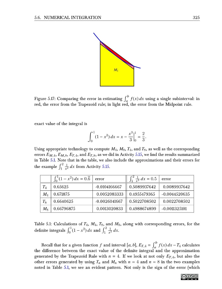
M 1
Figure 5.17: Comparing the error in estimating
b
a
f (x) dx using a single subinterval: in
red, the error from the Trapezoid rule; in light red, the error from the Midpoint rule.
exact value of the integral is
1
0
(1 − x
2 ) dx = x −
x 3
3
1
0
=
2
3
.
Using appropriate technology to compute M 4 , M 8 , T 4 , and T 8 , as well as the corresponding
errors E M,4 , E M,8 , E T,4 , and E T,8 , as we did in Activity 5.15, we find the results summarized
in Table 5.1. Note that in the table, we also include the approximations and their errors for
the example
2
1
1
x 2 dx from Activity 5.15.
1
0
(1 − x 2 ) dx = 0.6 error
2
1
1
x 2 dx = 0.5 error
T 4
0.65625
-0.0104166667
0.5089937642
0.0089937642
M 4 0.671875
0.0052083333 0.4955479365 -0.0044520635
T 8
0.6640625
-0.0026041667 0.5022708502
0.0022708502
M 8 0.66796875
0.0013020833 0.4988674899 -0.0011325101
Table 5.1: Calculations of T 4 , M 4 , T 8 , and M 8 , along with corresponding errors, for the
definite integrals
1
0
(1 − x 2 ) dx and
2
1
1
x 2 dx.
Recall that for a given function f and interval [a, b], E T,4 =
b
a
f (x) dx − T 4 calculates
the difference between the exact value of the definite integral and the approximation
generated by the Trapezoid Rule with n = 4. If we look at not only E T,4 , but also the
other errors generated by using T n and M n with n = 4 and n = 8 in the two examples
noted in Table 5.1, we see an evident pattern. Not only is the sign of the error (which
325
M 1
Figure 5.17: Comparing the error in estimating
b
a
f (x) dx using a single subinterval: in
red, the error from the Trapezoid rule; in light red, the error from the Midpoint rule.
exact value of the integral is
1
0
(1 − x
2 ) dx = x −
x 3
3
1
0
=
2
3
.
Using appropriate technology to compute M 4 , M 8 , T 4 , and T 8 , as well as the corresponding
errors E M,4 , E M,8 , E T,4 , and E T,8 , as we did in Activity 5.15, we find the results summarized
in Table 5.1. Note that in the table, we also include the approximations and their errors for
the example
2
1
1
x 2 dx from Activity 5.15.
1
0
(1 − x 2 ) dx = 0.6 error
2
1
1
x 2 dx = 0.5 error
T 4
0.65625
-0.0104166667
0.5089937642
0.0089937642
M 4 0.671875
0.0052083333 0.4955479365 -0.0044520635
T 8
0.6640625
-0.0026041667 0.5022708502
0.0022708502
M 8 0.66796875
0.0013020833 0.4988674899 -0.0011325101
Table 5.1: Calculations of T 4 , M 4 , T 8 , and M 8 , along with corresponding errors, for the
definite integrals
1
0
(1 − x 2 ) dx and
2
1
1
x 2 dx.
Recall that for a given function f and interval [a, b], E T,4 =
b
a
f (x) dx − T 4 calculates
the difference between the exact value of the definite integral and the approximation
generated by the Trapezoid Rule with n = 4. If we look at not only E T,4 , but also the
other errors generated by using T n and M n with n = 4 and n = 8 in the two examples
noted in Table 5.1, we see an evident pattern. Not only is the sign of the error (which