

324
5.6. NUMERICAL INTEGRATION
to patterns in errors, such as those observed in Activity 5.15, is one way to begin to see
some alternate approaches.
To begin, we make a comparison of the errors in the Midpoint and Trapezoid rules
from two different perspectives. First, consider a function of consistent concavity on a
given interval, and picture approximating the area bounded on that interval by both
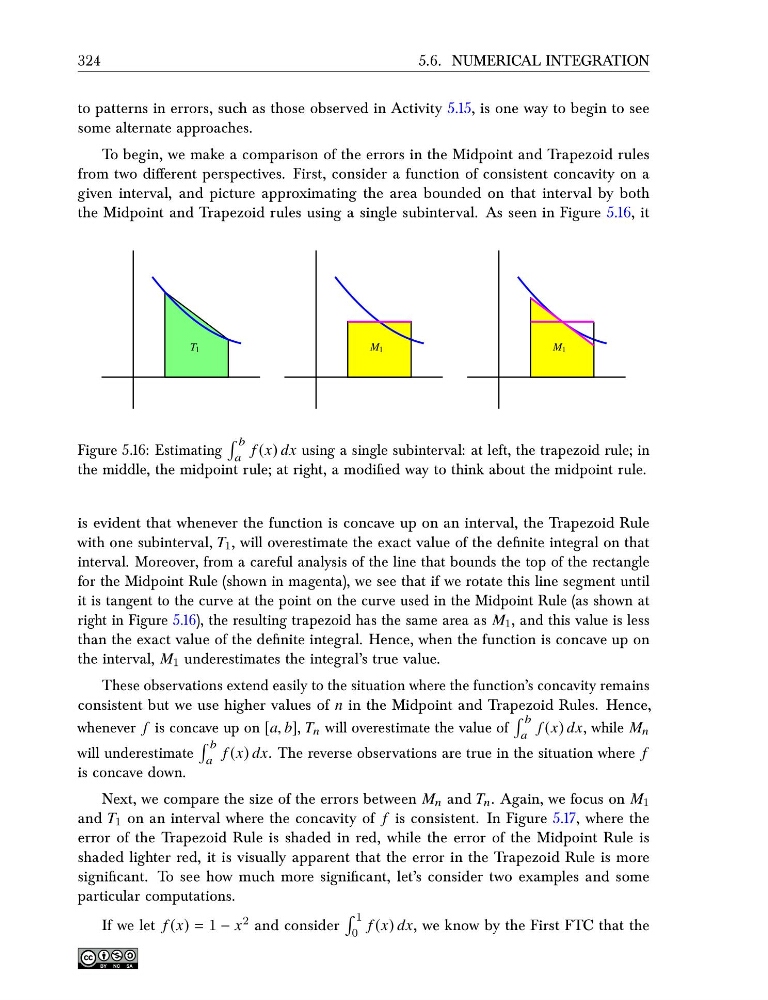
the Midpoint and Trapezoid rules using a single subinterval. As seen in Figure 5.16, it
T 1
M 1
M 1
Figure 5.16: Estimating
b
a
f (x) dx using a single subinterval: at left, the trapezoid rule; in
the middle, the midpoint rule; at right, a modified way to think about the midpoint rule.
is evident that whenever the function is concave up on an interval, the Trapezoid Rule
with one subinterval, T 1 , will overestimate the exact value of the definite integral on that
interval. Moreover, from a careful analysis of the line that bounds the top of the rectangle
for the Midpoint Rule (shown in magenta), we see that if we rotate this line segment until
it is tangent to the curve at the point on the curve used in the Midpoint Rule (as shown at
right in Figure 5.16), the resulting trapezoid has the same area as M 1 , and this value is less
than the exact value of the definite integral. Hence, when the function is concave up on
the interval, M 1 underestimates the integral’s true value.
These observations extend easily to the situation where the function’s concavity remains
consistent but we use higher values of n in the Midpoint and Trapezoid Rules. Hence,
whenever f is concave up on [a, b], T n will overestimate the value of
b
a
f (x) dx, while M n
will underestimate
b
a
f (x) dx. The reverse observations are true in the situation where f
is concave down.
Next, we compare the size of the errors between M n and T n . Again, we focus on M 1
and T 1 on an interval where the concavity of f is consistent. In Figure 5.17, where the
error of the Trapezoid Rule is shaded in red, while the error of the Midpoint Rule is
shaded lighter red, it is visually apparent that the error in the Trapezoid Rule is more
significant. To see how much more significant, let’s consider two examples and some
particular computations.
If we let f (x) = 1 − x 2 and consider
1
0
f (x) dx, we know by the First FTC that the
5.6. NUMERICAL INTEGRATION
to patterns in errors, such as those observed in Activity 5.15, is one way to begin to see
some alternate approaches.
To begin, we make a comparison of the errors in the Midpoint and Trapezoid rules
from two different perspectives. First, consider a function of consistent concavity on a
given interval, and picture approximating the area bounded on that interval by both
the Midpoint and Trapezoid rules using a single subinterval. As seen in Figure 5.16, it
T 1
M 1
M 1
Figure 5.16: Estimating
b
a
f (x) dx using a single subinterval: at left, the trapezoid rule; in
the middle, the midpoint rule; at right, a modified way to think about the midpoint rule.
is evident that whenever the function is concave up on an interval, the Trapezoid Rule
with one subinterval, T 1 , will overestimate the exact value of the definite integral on that
interval. Moreover, from a careful analysis of the line that bounds the top of the rectangle
for the Midpoint Rule (shown in magenta), we see that if we rotate this line segment until
it is tangent to the curve at the point on the curve used in the Midpoint Rule (as shown at
right in Figure 5.16), the resulting trapezoid has the same area as M 1 , and this value is less
than the exact value of the definite integral. Hence, when the function is concave up on
the interval, M 1 underestimates the integral’s true value.
These observations extend easily to the situation where the function’s concavity remains
consistent but we use higher values of n in the Midpoint and Trapezoid Rules. Hence,
whenever f is concave up on [a, b], T n will overestimate the value of
b
a
f (x) dx, while M n
will underestimate
b
a
f (x) dx. The reverse observations are true in the situation where f
is concave down.
Next, we compare the size of the errors between M n and T n . Again, we focus on M 1
and T 1 on an interval where the concavity of f is consistent. In Figure 5.17, where the
error of the Trapezoid Rule is shaded in red, while the error of the Midpoint Rule is
shaded lighter red, it is visually apparent that the error in the Trapezoid Rule is more
significant. To see how much more significant, let’s consider two examples and some
particular computations.
If we let f (x) = 1 − x 2 and consider
1
0
f (x) dx, we know by the First FTC that the