

1.2. THE NOTION OF LIMIT
15
to its function value. Here, it follows that as x → −1, (4 − x 2 ) → (4 − (−1) 2 ) = 3, and
(x + 2) → (−1 + 2) = 1, so as x → −1, the numerator of f tends to 3 and the denominator
tends to 1, hence lim
x→−1
f (x) =
3
1
= 3.
The situation is more complicated when x → −2, due in part to the fact that f (−2) is
not defined. If we attempt to use a similar algebraic argument regarding the numerator
and denominator, we observe that as x → −2, (4 − x 2 ) → (4 − (−2) 2 ) = 0, and (x + 2) →
(−2 + 2) = 0, so as x → −2, the numerator of f tends to 0 and the denominator tends to
0. We call 0/0 an indeterminate form and will revisit several important issues surrounding
such quantities later in the course. For now, we simply observe that this tells us there is
somehow more work to do. From the table and the graph, it appears that f should have a
limit of 4 at x = −2. To see algebraically why this is the case, let’s work directly with the
form of f (x). Observe that
lim
x→−2
f (x) = lim
x→−2
4 − x 2
x + 2
= lim
x→−2
(2 − x)(2 + x)
x + 2
.
At this point, it is important to observe that since we are taking the limit as x → −2, we
are considering x values that are close, but not equal, to −2. Since we never actually allow
x to equal −2, the quotient
2+x
x+2 has value 1 for every possible value of x. Thus, we can
simplify the most recent expression above, and now find that
lim
x→−2
f (x) = lim
x→−2
2 − x.
Because 2 − x is simply a linear function, this limit is now easy to determine, and its value
clearly is 4. Thus, from several points of view we’ve seen that lim
x→−2
f (x) = 4.
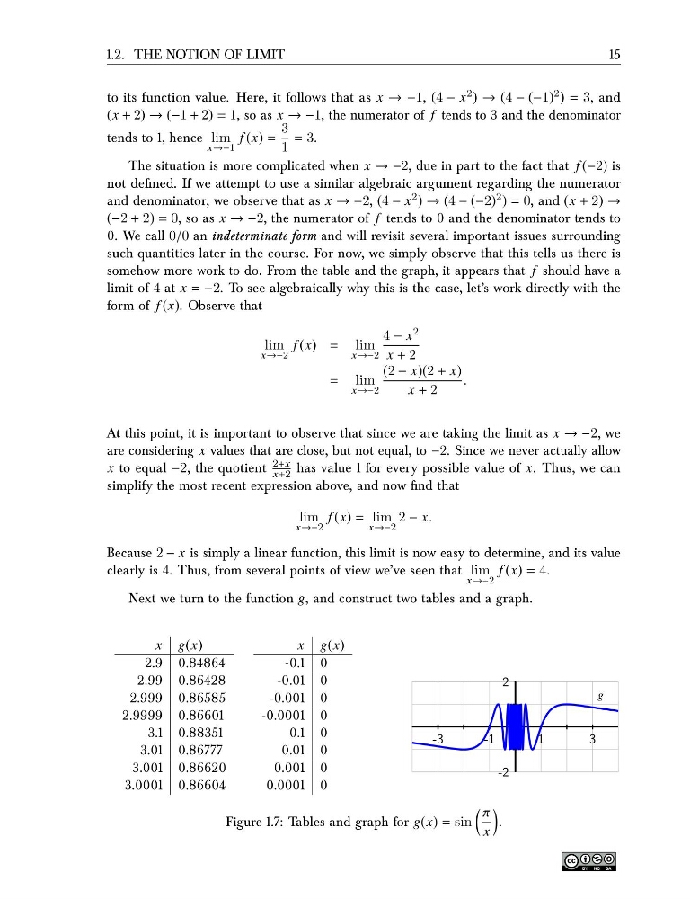
Next we turn to the function g, and construct two tables and a graph.
x g(x)
2.9 0.84864
2.99 0.86428
2.999 0.86585
2.9999 0.86601
3.1 0.88351
3.01 0.86777
3.001 0.86620
3.0001 0.86604
x g(x)
-0.1 0
-0.01 0
-0.001 0
-0.0001 0
0.1 0
0.01 0
0.001 0
0.0001 0
-3
-1
1
3
-2
2
g
Figure 1.7: Tables and graph for g(x) = sin
π
x
.
15
to its function value. Here, it follows that as x → −1, (4 − x 2 ) → (4 − (−1) 2 ) = 3, and
(x + 2) → (−1 + 2) = 1, so as x → −1, the numerator of f tends to 3 and the denominator
tends to 1, hence lim
x→−1
f (x) =
3
1
= 3.
The situation is more complicated when x → −2, due in part to the fact that f (−2) is
not defined. If we attempt to use a similar algebraic argument regarding the numerator
and denominator, we observe that as x → −2, (4 − x 2 ) → (4 − (−2) 2 ) = 0, and (x + 2) →
(−2 + 2) = 0, so as x → −2, the numerator of f tends to 0 and the denominator tends to
0. We call 0/0 an indeterminate form and will revisit several important issues surrounding
such quantities later in the course. For now, we simply observe that this tells us there is
somehow more work to do. From the table and the graph, it appears that f should have a
limit of 4 at x = −2. To see algebraically why this is the case, let’s work directly with the
form of f (x). Observe that
lim
x→−2
f (x) = lim
x→−2
4 − x 2
x + 2
= lim
x→−2
(2 − x)(2 + x)
x + 2
.
At this point, it is important to observe that since we are taking the limit as x → −2, we
are considering x values that are close, but not equal, to −2. Since we never actually allow
x to equal −2, the quotient
2+x
x+2 has value 1 for every possible value of x. Thus, we can
simplify the most recent expression above, and now find that
lim
x→−2
f (x) = lim
x→−2
2 − x.
Because 2 − x is simply a linear function, this limit is now easy to determine, and its value
clearly is 4. Thus, from several points of view we’ve seen that lim
x→−2
f (x) = 4.
Next we turn to the function g, and construct two tables and a graph.
x g(x)
2.9 0.84864
2.99 0.86428
2.999 0.86585
2.9999 0.86601
3.1 0.88351
3.01 0.86777
3.001 0.86620
3.0001 0.86604
x g(x)
-0.1 0
-0.01 0
-0.001 0
-0.0001 0
0.1 0
0.01 0
0.001 0
0.0001 0
-3
-1
1
3
-2
2
g
Figure 1.7: Tables and graph for g(x) = sin
π
x
.