

14
1.2. THE NOTION OF LIMIT
often be used to determine the limit exactly. The following example demonstrates both of
these approaches, while also using the graphs of the respective functions to help confirm
our conclusions.
Example 1.2. For each of the following functions, we’ d like to know whether or not the
function has a limit at the stated a-values. Use both numerical and algebraic approaches
to investigate and, if possible, estimate or determine the value of the limit. Compare the
results with a careful graph of the function on an interval containing the points of interest.
(a) f (x) =
4 − x 2
x + 2
; a = −1, a = −2
(b) g(x) = sin
π
x
; a = 3, a = 0
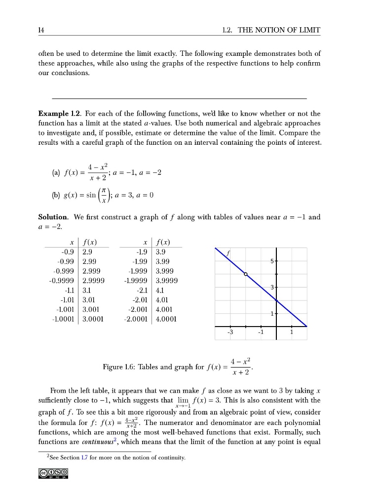
Solution. We first construct a graph of f along with tables of values near a = −1 and
a = −2.
x f (x)
-0.9 2.9
-0.99 2.99
-0.999 2.999
-0.9999 2.9999
-1.1 3.1
-1.01 3.01
-1.001 3.001
-1.0001 3.0001
x f (x)
-1.9 3.9
-1.99 3.99
-1.999 3.999
-1.9999 3.9999
-2.1 4.1
-2.01 4.01
-2.001 4.001
-2.0001 4.0001
-3
-1
1
1
3
5
f
Figure 1.6: Tables and graph for f (x) =
4 − x 2
x + 2
.
From the left table, it appears that we can make f as close as we want to 3 by taking x
sufficiently close to −1, which suggests that lim
x→−1
f (x) = 3. This is also consistent with the
graph of f . To see this a bit more rigorously and from an algebraic point of view, consider
the formula for f : f (x) =
4−x 2
x+2 . The numerator and denominator are each polynomial
functions, which are among the most well-behaved functions that exist. Formally, such
functions are continuous 2 , which means that the limit of the function at any point is equal
2 See Section 1.7 for more on the notion of continuity.
1.2. THE NOTION OF LIMIT
often be used to determine the limit exactly. The following example demonstrates both of
these approaches, while also using the graphs of the respective functions to help confirm
our conclusions.
Example 1.2. For each of the following functions, we’ d like to know whether or not the
function has a limit at the stated a-values. Use both numerical and algebraic approaches
to investigate and, if possible, estimate or determine the value of the limit. Compare the
results with a careful graph of the function on an interval containing the points of interest.
(a) f (x) =
4 − x 2
x + 2
; a = −1, a = −2
(b) g(x) = sin
π
x
; a = 3, a = 0
Solution. We first construct a graph of f along with tables of values near a = −1 and
a = −2.
x f (x)
-0.9 2.9
-0.99 2.99
-0.999 2.999
-0.9999 2.9999
-1.1 3.1
-1.01 3.01
-1.001 3.001
-1.0001 3.0001
x f (x)
-1.9 3.9
-1.99 3.99
-1.999 3.999
-1.9999 3.9999
-2.1 4.1
-2.01 4.01
-2.001 4.001
-2.0001 4.0001
-3
-1
1
1
3
5
f
Figure 1.6: Tables and graph for f (x) =
4 − x 2
x + 2
.
From the left table, it appears that we can make f as close as we want to 3 by taking x
sufficiently close to −1, which suggests that lim
x→−1
f (x) = 3. This is also consistent with the
graph of f . To see this a bit more rigorously and from an algebraic point of view, consider
the formula for f : f (x) =
4−x 2
x+2 . The numerator and denominator are each polynomial
functions, which are among the most well-behaved functions that exist. Formally, such
functions are continuous 2 , which means that the limit of the function at any point is equal
2 See Section 1.7 for more on the notion of continuity.