

5.1. CONSTRUCTING ACCURATE GRAPHS OF ANTIDERIVATIVES
269
(e) Based on your responses to all of the preceding questions, sketch a complete
and accurate graph of y = F(x) on the axes provided, being sure to indicate
the behavior of F for x < 0 and x > 7. Clearly indicate the scale on the vertical
and horizontal axes of your graph.
(f) What happens if we change one key piece of information: in particular, say that
G is an antiderivative of f and G(0) = 0. How (if at all) would your answers to
the preceding questions change? Sketch a graph of G on the same axes as the
graph of F you constructed in (e).
⊳
Multiple antiderivatives of a single function
In the final question of Activity 5.1, we encountered a very important idea: a given function
f has more than one antiderivative. In addition, any antiderivative of f is determined
uniquely by identifying the value of the desired antiderivative at a single point. For
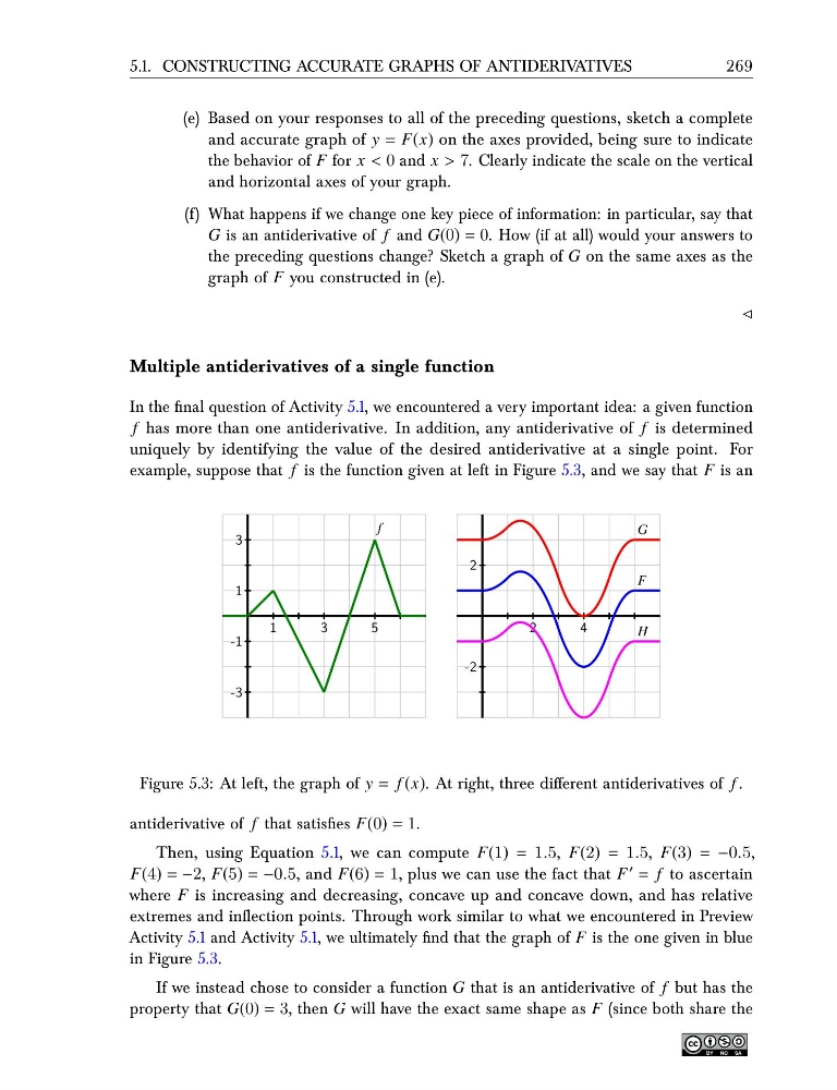
example, suppose that f is the function given at left in Figure 5.3, and we say that F is an
1
3
5
-3
-1
1
3
f
2
4
-2
2
F
G
H
Figure 5.3: At left, the graph of y = f (x). At right, three different antiderivatives of f .
antiderivative of f that satisfies F(0) = 1.
Then, using Equation 5.1, we can compute F(1) = 1.5, F(2) = 1.5, F(3) = −0.5,
F(4) = −2, F(5) = −0.5, and F(6) = 1, plus we can use the fact that F ′ = f to ascertain
where F is increasing and decreasing, concave up and concave down, and has relative
extremes and inflection points. Through work similar to what we encountered in Preview
Activity 5.1 and Activity 5.1, we ultimately find that the graph of F is the one given in blue
in Figure 5.3.
If we instead chose to consider a function G that is an antiderivative of f but has the
property that G(0) = 3, then G will have the exact same shape as F (since both share the
269
(e) Based on your responses to all of the preceding questions, sketch a complete
and accurate graph of y = F(x) on the axes provided, being sure to indicate
the behavior of F for x < 0 and x > 7. Clearly indicate the scale on the vertical
and horizontal axes of your graph.
(f) What happens if we change one key piece of information: in particular, say that
G is an antiderivative of f and G(0) = 0. How (if at all) would your answers to
the preceding questions change? Sketch a graph of G on the same axes as the
graph of F you constructed in (e).
⊳
Multiple antiderivatives of a single function
In the final question of Activity 5.1, we encountered a very important idea: a given function
f has more than one antiderivative. In addition, any antiderivative of f is determined
uniquely by identifying the value of the desired antiderivative at a single point. For
example, suppose that f is the function given at left in Figure 5.3, and we say that F is an
1
3
5
-3
-1
1
3
f
2
4
-2
2
F
G
H
Figure 5.3: At left, the graph of y = f (x). At right, three different antiderivatives of f .
antiderivative of f that satisfies F(0) = 1.
Then, using Equation 5.1, we can compute F(1) = 1.5, F(2) = 1.5, F(3) = −0.5,
F(4) = −2, F(5) = −0.5, and F(6) = 1, plus we can use the fact that F ′ = f to ascertain
where F is increasing and decreasing, concave up and concave down, and has relative
extremes and inflection points. Through work similar to what we encountered in Preview
Activity 5.1 and Activity 5.1, we ultimately find that the graph of F is the one given in blue
in Figure 5.3.
If we instead chose to consider a function G that is an antiderivative of f but has the
property that G(0) = 3, then G will have the exact same shape as F (since both share the