

4.2. RIEMANN SUMS
227
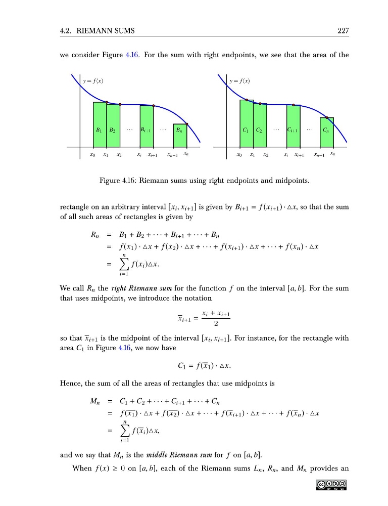
we consider Figure 4.16. For the sum with right endpoints, we see that the area of the
x 0 x 1 x 2
x i x i+1
x n−1 x n
B 1 B 2
· · · B i+1
· · ·
y = f (x)
B n
x 0 x 1 x 2
x i x i+1
x n−1 x n
C 1 C 2
· · · C i+1
· · ·
y = f (x)
C n
Figure 4.16: Riemann sums using right endpoints and midpoints.
rectangle on an arbitrary interval [x i , x i+1 ] is given by B i+1 = f (x i+1 ) · △x, so that the sum
of all such areas of rectangles is given by
R n = B 1 + B 2 + · · · + B i+1 + · · · + B n
= f (x 1 ) · △x + f (x 2 ) · △x + · · · + f (x i+1 ) · △x + · · · + f (x n ) · △x
=
n
i=1
f (x i )△x.
We call R n the right Riemann sum for the function f on the interval [a, b]. For the sum
that uses midpoints, we introduce the notation
x i+1 =
x i + x i+1
2
so that x i+1 is the midpoint of the interval [x i , x i+1 ]. For instance, for the rectangle with
area C 1 in Figure 4.16, we now have
C 1 = f (x 1 ) · △x.
Hence, the sum of all the areas of rectangles that use midpoints is
M n = C 1 + C 2 + · · · + C i+1 + · · · + C n
= f (x 1 ) · △x + f (x 2 ) · △x + · · · + f (x i+1 ) · △x + · · · + f (x n ) · △x
=
n
i=1
f (x i )△x,
and we say that M n is the middle Riemann sum for f on [a, b].
When f (x) ≥ 0 on [a, b], each of the Riemann sums L n , R n , and M n provides an
227
we consider Figure 4.16. For the sum with right endpoints, we see that the area of the
x 0 x 1 x 2
x i x i+1
x n−1 x n
B 1 B 2
· · · B i+1
· · ·
y = f (x)
B n
x 0 x 1 x 2
x i x i+1
x n−1 x n
C 1 C 2
· · · C i+1
· · ·
y = f (x)
C n
Figure 4.16: Riemann sums using right endpoints and midpoints.
rectangle on an arbitrary interval [x i , x i+1 ] is given by B i+1 = f (x i+1 ) · △x, so that the sum
of all such areas of rectangles is given by
R n = B 1 + B 2 + · · · + B i+1 + · · · + B n
= f (x 1 ) · △x + f (x 2 ) · △x + · · · + f (x i+1 ) · △x + · · · + f (x n ) · △x
=
n
i=1
f (x i )△x.
We call R n the right Riemann sum for the function f on the interval [a, b]. For the sum
that uses midpoints, we introduce the notation
x i+1 =
x i + x i+1
2
so that x i+1 is the midpoint of the interval [x i , x i+1 ]. For instance, for the rectangle with
area C 1 in Figure 4.16, we now have
C 1 = f (x 1 ) · △x.
Hence, the sum of all the areas of rectangles that use midpoints is
M n = C 1 + C 2 + · · · + C i+1 + · · · + C n
= f (x 1 ) · △x + f (x 2 ) · △x + · · · + f (x i+1 ) · △x + · · · + f (x n ) · △x
=
n
i=1
f (x i )△x,
and we say that M n is the middle Riemann sum for f on [a, b].
When f (x) ≥ 0 on [a, b], each of the Riemann sums L n , R n , and M n provides an