

222
4.2. RIEMANN SUMS
while the total change in the object’s position on [a, b] is
s(b) − s(a) = A 1 − A 2 + A 3 .
Because the motion is in the negative direction on the interval where v(t) < 0, we subtract
A 2 when determining the object’s total change in position.
Of course, finding D and s(b) − s(a) for the situation given in Figure 4.11 presumes
that we can actually find the areas represented by A 1 , A 2 , and A 3 . In most of our work in
Section 4.1, such as in Activities 4.2 and 4.3, we worked with velocity functions that were
either constant or linear, so that by finding the areas of rectangles and triangles, we could
find the area bounded by the velocity function and the horizontal axis exactly. But when
the curve that bounds a region is not one for which we have a known formula for area, we
are unable to find this area exactly. Indeed, this is one of our biggest goals in Chapter 4:
to learn how to find the exact area bounded between a curve and the horizontal axis for
as many different types of functions as possible.
To begin, we expand on the ideas in Activity 4.1, where we encountered a nonlinear
velocity function and approximated the area under the curve using four and eight rectangles,
respectively. In the following preview activity, we focus on three different options for
deciding how to find the heights of the rectangles we will use.
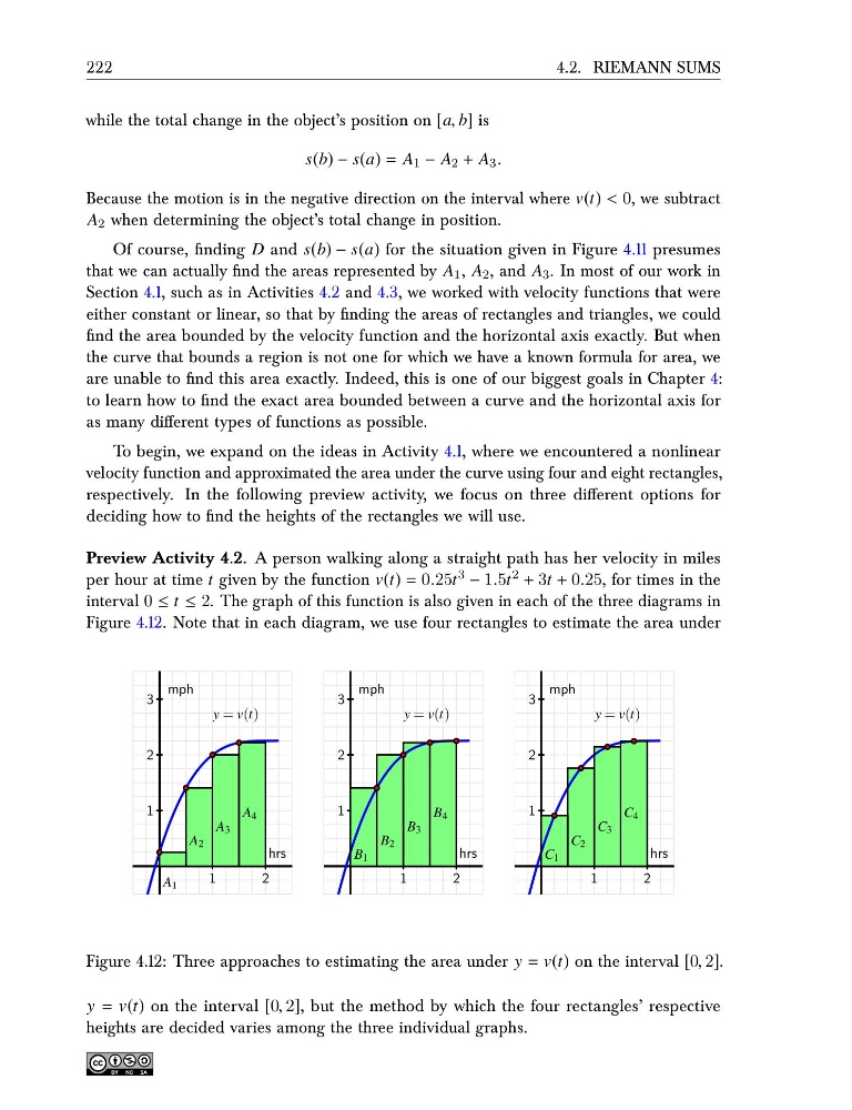
Preview Activity 4.2. A person walking along a straight path has her velocity in miles
per hour at time t given by the function v(t) = 0.25t 3 − 1.5t 2 + 3t + 0.25, for times in the
interval 0 ≤ t ≤ 2. The graph of this function is also given in each of the three diagrams in
Figure 4.12. Note that in each diagram, we use four rectangles to estimate the area under
1
2
1
2
3
mph
hrs
y = v(t)
A 1
A 2
A 3
A 4
1
2
1
2
3
mph
hrs
y = v(t)
B 1
B 2
B 3
B 4
1
2
1
2
3
mph
hrs
y = v(t)
C 1
C 2
C 3
C 4
Figure 4.12: Three approaches to estimating the area under y = v(t) on the interval [0, 2].
y = v(t) on the interval [0, 2], but the method by which the four rectangles’ respective
heights are decided varies among the three individual graphs.
4.2. RIEMANN SUMS
while the total change in the object’s position on [a, b] is
s(b) − s(a) = A 1 − A 2 + A 3 .
Because the motion is in the negative direction on the interval where v(t) < 0, we subtract
A 2 when determining the object’s total change in position.
Of course, finding D and s(b) − s(a) for the situation given in Figure 4.11 presumes
that we can actually find the areas represented by A 1 , A 2 , and A 3 . In most of our work in
Section 4.1, such as in Activities 4.2 and 4.3, we worked with velocity functions that were
either constant or linear, so that by finding the areas of rectangles and triangles, we could
find the area bounded by the velocity function and the horizontal axis exactly. But when
the curve that bounds a region is not one for which we have a known formula for area, we
are unable to find this area exactly. Indeed, this is one of our biggest goals in Chapter 4:
to learn how to find the exact area bounded between a curve and the horizontal axis for
as many different types of functions as possible.
To begin, we expand on the ideas in Activity 4.1, where we encountered a nonlinear
velocity function and approximated the area under the curve using four and eight rectangles,
respectively. In the following preview activity, we focus on three different options for
deciding how to find the heights of the rectangles we will use.
Preview Activity 4.2. A person walking along a straight path has her velocity in miles
per hour at time t given by the function v(t) = 0.25t 3 − 1.5t 2 + 3t + 0.25, for times in the
interval 0 ≤ t ≤ 2. The graph of this function is also given in each of the three diagrams in
Figure 4.12. Note that in each diagram, we use four rectangles to estimate the area under
1
2
1
2
3
mph
hrs
y = v(t)
A 1
A 2
A 3
A 4
1
2
1
2
3
mph
hrs
y = v(t)
B 1
B 2
B 3
B 4
1
2
1
2
3
mph
hrs
y = v(t)
C 1
C 2
C 3
C 4
Figure 4.12: Three approaches to estimating the area under y = v(t) on the interval [0, 2].
y = v(t) on the interval [0, 2], but the method by which the four rectangles’ respective
heights are decided varies among the three individual graphs.