

4.2. RIEMANN SUMS
221
4.2 Riemann Sums
Motivating Questions
In this section, we strive to understand the ideas generated by the following important
questions:
• How can we use a Riemann sum to estimate the area between a given curve and
the horizontal axis over a particular interval?
• What are the differences among left, right, middle, and random Riemann sums?
• How can we write Riemann sums in an abbreviated form??
Introduction
In Section 4.1, we learned that if we have a moving object with velocity function v, whenever
v(t) is positive, the area between y = v(t) and the t-axis over a given time interval tells us
the distance traveled by the object over that time period; in addition, if v(t) is sometimes
negative and we view the area of any region below the t-axis as having an associated
negative sign, then the sum of these signed areas over a given interval tells us the moving
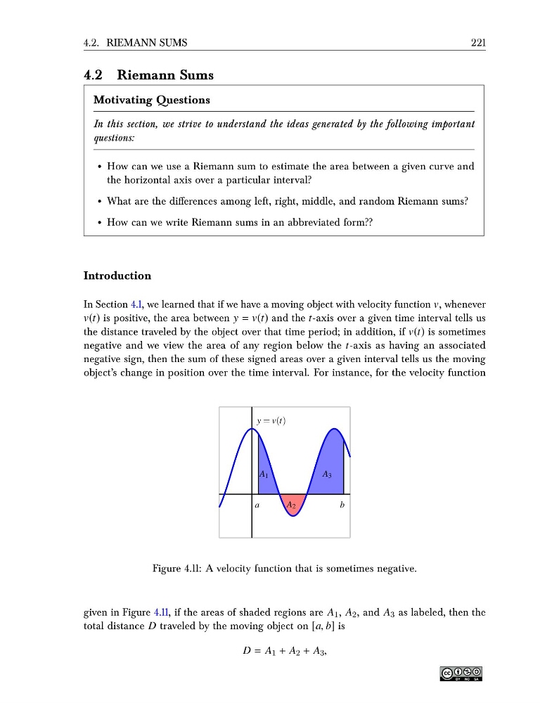
object’s change in position over the time interval. For instance, for the velocity function
y = v(t)
a
b
A 1
A 2
A 3
Figure 4.11: A velocity function that is sometimes negative.
given in Figure 4.11, if the areas of shaded regions are A 1 , A 2 , and A 3 as labeled, then the
total distance D traveled by the moving object on [a, b] is
D = A 1 + A 2 + A 3 ,
221
4.2 Riemann Sums
Motivating Questions
In this section, we strive to understand the ideas generated by the following important
questions:
• How can we use a Riemann sum to estimate the area between a given curve and
the horizontal axis over a particular interval?
• What are the differences among left, right, middle, and random Riemann sums?
• How can we write Riemann sums in an abbreviated form??
Introduction
In Section 4.1, we learned that if we have a moving object with velocity function v, whenever
v(t) is positive, the area between y = v(t) and the t-axis over a given time interval tells us
the distance traveled by the object over that time period; in addition, if v(t) is sometimes
negative and we view the area of any region below the t-axis as having an associated
negative sign, then the sum of these signed areas over a given interval tells us the moving
object’s change in position over the time interval. For instance, for the velocity function
y = v(t)
a
b
A 1
A 2
A 3
Figure 4.11: A velocity function that is sometimes negative.
given in Figure 4.11, if the areas of shaded regions are A 1 , A 2 , and A 3 as labeled, then the
total distance D traveled by the moving object on [a, b] is
D = A 1 + A 2 + A 3 ,