

52
GAUGE FIELDS AND STRINGS
and with this knowledge we can proceed to calculate the one kink
contribution to the correlation function:
^^0 ^clih ~ ^o)^c\i^2 ~ ^o)
1 -h ß e
A
|d t„
^^0 (^cl (tl ~ to)(/>ci(t2 ~ to) —
(4.14)
ß = A J ----------------ndi„e-^
Substituting (4.6) into (4.14) we obtain:
<
C= -B
2B
C /
ux
u(x — 1)
dx j tanh ^ \t^ — t2 \ tanh---- — |ii — ^2! “ 1
V2 '
Ui - ^2! > ^ ^
V2
(4.15)
As was expected, for large times the kink solution (4.6) gives a large
contribution. Moreover, it is clear that we have to take into account
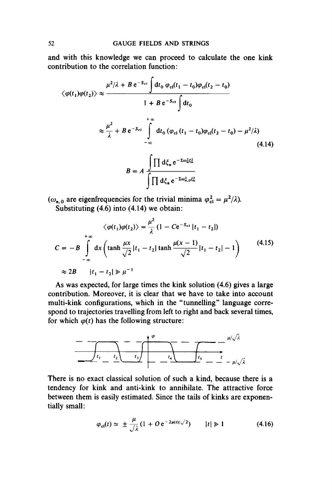
multi-kink configurations, which in the “tunnelling” language correspond to trajectories travelling from left to right and back several times,
for which (p(t) has the following structure:
It,
t.
h
t
r
--------- --- 1 ^ 1
There is no exact classical solution of such a kind, because there is a
tendency for kink and anti-kink to annihilate. The attractive force
between them is easily estimated. Since the tails of kinks are exponentially small:
(
1
\t\>l
(4.16)
GAUGE FIELDS AND STRINGS
and with this knowledge we can proceed to calculate the one kink
contribution to the correlation function:
^^0 ^clih ~ ^o)^c\i^2 ~ ^o)
1 -h ß e
A
|d t„
^^0 (^cl (tl ~ to)(/>ci(t2 ~ to) —
(4.14)
ß = A J ----------------ndi„e-^
Substituting (4.6) into (4.14) we obtain:
<
C= -B
2B
C /
ux
u(x — 1)
dx j tanh ^ \t^ — t2 \ tanh---- — |ii — ^2! “ 1
V2 '
Ui - ^2! > ^ ^
V2
(4.15)
As was expected, for large times the kink solution (4.6) gives a large
contribution. Moreover, it is clear that we have to take into account
multi-kink configurations, which in the “tunnelling” language correspond to trajectories travelling from left to right and back several times,
for which (p(t) has the following structure:
It,
t.
h
t
r
--------- --- 1 ^ 1
There is no exact classical solution of such a kind, because there is a
tendency for kink and anti-kink to annihilate. The attractive force
between them is easily estimated. Since the tails of kinks are exponentially small:
(
1
\t\>l
(4.16)