

50
GAUGE FIELDS AND STRINGS
restored symmetry. It is clear that restoration of symmetry occurs
because a particle placed in the left well will (with finite probability)
tunnel to the right one and back. Therefore if we wait long enough there
will be equal probability of finding the particle in either of the wells.
There exists an interesting way to describe tunnelling which we briefly
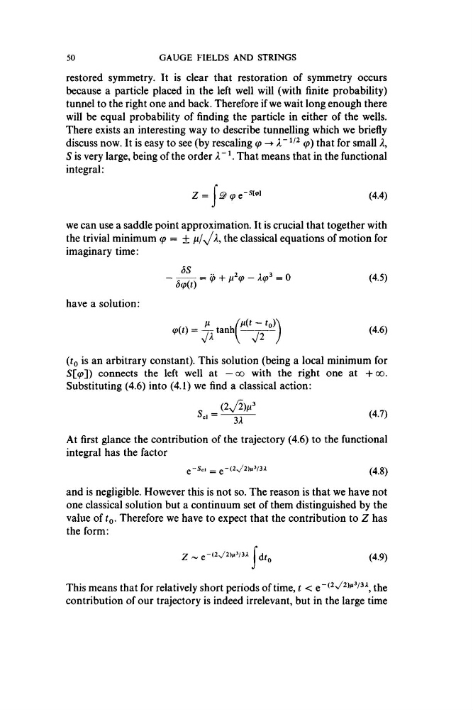
discuss now. It is easy to see (by rescaling q >
q> ) that for small X,
S is very large, being of the order A" ^ That means that in the functional
integral:
Z = ^ (pe -S[
we can use a saddle point approximation. It is crucial that together with
the trivial minimum < p = ±
the classical equations of motion for
imaginary time:
Sq)(t)
= (p p L ^cp — X cp^ = 0
have a solution:
(4.5)
(4.6)
(io is an arbitrary constant). This solution (being a local minimum for
5[(p]) connects the left well at — oo with the right one at +oo.
Substituting (4.6) into (4.1) we find a classical action:
^cl ~ 3A
(4.7)
At first glance the contribution of the trajectory (4.6) to the functional
integral has the factor
g - S c i _ q-(2^2)h^ I3X
(4 8)
and is negligible. However this is not so. The reason is that we have not
one classical solution but a continuum set of them distinguished by the
value of ìq- Therefore we have to expect that the contribution to Z has
the form:
-(2v/2)m V 3A jdio
(4.9)
This means that for relatively short periods of time, t < e (2v/2)ii3/3A ^
contribution of our trajectory is indeed irrelevant, but in the large time
GAUGE FIELDS AND STRINGS
restored symmetry. It is clear that restoration of symmetry occurs
because a particle placed in the left well will (with finite probability)
tunnel to the right one and back. Therefore if we wait long enough there
will be equal probability of finding the particle in either of the wells.
There exists an interesting way to describe tunnelling which we briefly
discuss now. It is easy to see (by rescaling q >
q> ) that for small X,
S is very large, being of the order A" ^ That means that in the functional
integral:
Z = ^ (pe -S[
we can use a saddle point approximation. It is crucial that together with
the trivial minimum < p = ±
the classical equations of motion for
imaginary time:
Sq)(t)
= (p p L ^cp — X cp^ = 0
have a solution:
(4.5)
(4.6)
(io is an arbitrary constant). This solution (being a local minimum for
5[(p]) connects the left well at — oo with the right one at +oo.
Substituting (4.6) into (4.1) we find a classical action:
^cl ~ 3A
(4.7)
At first glance the contribution of the trajectory (4.6) to the functional
integral has the factor
g - S c i _ q-(2^2)h^ I3X
(4 8)
and is negligible. However this is not so. The reason is that we have not
one classical solution but a continuum set of them distinguished by the
value of ìq- Therefore we have to expect that the contribution to Z has
the form:
-(2v/2)m V 3A jdio
(4.9)
This means that for relatively short periods of time, t < e (2v/2)ii3/3A ^
contribution of our trajectory is indeed irrelevant, but in the large time