

ATTEMPT AT A SYNTHESIS
255
is renormalizable in the following sense. Suppose, that we integrate over
fast components of the x-field, with wave vectors lying between A and
A. As we will show now, the result will again be an action of the form
(10.6) but with a renormalized metric tensor
So, the set of all
possible
plays the role of the coupling constants in more ordinary
theories. In particular the nonlinear a-models, considered in the
beginning of the book, correspond to the special case when y^v(jc) are
taken to have constant curvature (this constraint is reproduced under
renormalization). The coupling constants which we have introduced
before are nothing but the values of these constant curvatures.
The computation begins, as usual, with the decomposition into fast y
and slow jCo parts of the field:
x(i) = Xo(0+y{0
Substituting (10.7) into (10.6) we obtain:
5(x) = S{xo) -h Sn(xQ,y)
(10.7)
( 10.8)
where Sh(xq, y) is quadratic in y. Linear terms in y are absent, because
they are of the form:
Si(xo,y) =
SS
Sx.
(10.9)
and while SS/Sxq contains wave vectors < A, wave vectors oiy lie in the
range from A to A. Hence, with our accuracy, the integral (10.9) is zero.
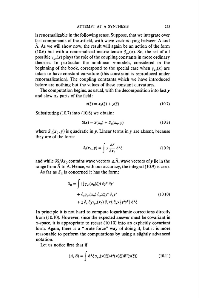
As far as S',, is concerned it has the form:
— j*
( 10.10)
In principle it is not hard to compute logarithmic corrections directly
from (10.10). However, since the expected answer must be covariant in
x-space, it is appropriate to recast (10.10) into an explicitly covariant
form. Again, there is a “brute force” way of doing it, but it is more
reasonable to perform the computations by using a slightly advanced
notation.
Let us notice first that if
(A, B ) = I dH
(10.11)
255
is renormalizable in the following sense. Suppose, that we integrate over
fast components of the x-field, with wave vectors lying between A and
A. As we will show now, the result will again be an action of the form
(10.6) but with a renormalized metric tensor
So, the set of all
possible
plays the role of the coupling constants in more ordinary
theories. In particular the nonlinear a-models, considered in the
beginning of the book, correspond to the special case when y^v(jc) are
taken to have constant curvature (this constraint is reproduced under
renormalization). The coupling constants which we have introduced
before are nothing but the values of these constant curvatures.
The computation begins, as usual, with the decomposition into fast y
and slow jCo parts of the field:
x(i) = Xo(0+y{0
Substituting (10.7) into (10.6) we obtain:
5(x) = S{xo) -h Sn(xQ,y)
(10.7)
( 10.8)
where Sh(xq, y) is quadratic in y. Linear terms in y are absent, because
they are of the form:
Si(xo,y) =
SS
Sx.
(10.9)
and while SS/Sxq contains wave vectors < A, wave vectors oiy lie in the
range from A to A. Hence, with our accuracy, the integral (10.9) is zero.
As far as S',, is concerned it has the form:
— j*
( 10.10)
In principle it is not hard to compute logarithmic corrections directly
from (10.10). However, since the expected answer must be covariant in
x-space, it is appropriate to recast (10.10) into an explicitly covariant
form. Again, there is a “brute force” way of doing it, but it is more
reasonable to perform the computations by using a slightly advanced
notation.
Let us notice first that if
(A, B ) = I dH
(10.11)