STATISTICAL MECHANICS AND QUANTUM FIELD THEORY
11
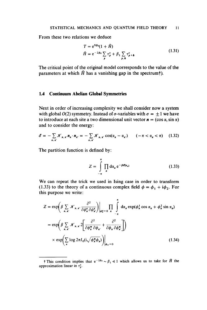
From these two relations we deduce
T =
+ H)
(1.31)
''y '
''j-i
y
j’.s
The critical point of the original model corresponds to the value of the
parameters at which H has a vanishing gap in the spectrumt).
1.4 Continuum Abelian Global Symmetries
Next in order of increasing complexity we shall consider now a system
with global 0(2) symmetry. Instead of a-variables with cr = ± 1 we have
to introduce at each site a two dimensional unit vector n = (cos a, sin a)
and to consider the energy:
^ = - Z
= - Z -^x.x' cos(a, - a,0
( - 7T < a, < 7r) (1.32)
The partition function is defined by:
n
(1.33)
We can repeat the trick we used in Ising case in order to transform
(1.33) to the theory of a continuous complex field (f) = (f)^ i(/)2. For
this purpose we write:
n
< t> ° = 0 X •
da, exp((/>^ cos a, -h (f>l sin a,)
= expi)S I
\
X, x'
(5^
+
d.. d4>,d.t>*
X ex p (x log 2n¡o (i^
(1.34)
t This condition implies that e
~
1 which allows us to take for A the
approximation linear in tJ.