

10
GAUGE FIELDS AND STRINGS
the lattice spacing by fixing the value of the so-called block-spins (e.g.,
we fix the sum of the spins occupying the vertices of each hypercube of
our lattice) and then summing over configurations with those fixed
values. As a result, we obtain an effective energy that depends on the
block-spins S', which are no longer restricted by S^ = 1. Repeating this
transformation many times we shall eventually come to an effective
action depending on a continuum field cp.
There is a tendency in particle physics to consider Lagrangians like
(1.25) as fundamental. It seems to me that it is more appropriate to
imagine some kind of a-like variables at very small distances, because
they carry a quintessence of the symmetry properties. This difference,
however, is not noticeable at large distances, and a theory of small
distances (of order the Planck length) still does not exist. The last thing
about the Ising model that we need to discuss in this preliminary
section is its Hamiltonian form. In order to derive it, let us split the ^ -
dimensional coordinate x into a ^ — 1 dimensional y and one “time”
dimension V.x =
Let us chose the coupling in the time direction to
be much stronger than in the space ones (universality should permit us
to play this trick without changing the critical properties). We have:
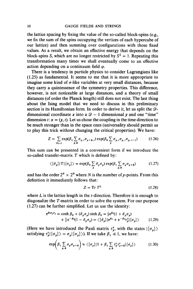
z = Zexp(^i
(1.26)
This sum can be presented in a convenient form if we introduce the
so-called transfer-matrix T which is defined by:
I
= expO?o z
exp(;8, Z (Ty(^y+»)
(1.27)
and has the order 2^ x 2^ where N is the number of j-points. From this
definition it immediately follows that:
Z = Tr
(1.28)
where L is the lattice length in the i-direction. Therefore it is enough to
diagonalize the T-matrix in order to solve the system. For our purpose
(1.27) can be further simplified. Let us use the identity:
^
(^y
(Here we have introduced the Pauli matrix tJ, with the states
satisfying Tl\{ay}y =
If we take
1, we have:
exp( Z
(1-30)
GAUGE FIELDS AND STRINGS
the lattice spacing by fixing the value of the so-called block-spins (e.g.,
we fix the sum of the spins occupying the vertices of each hypercube of
our lattice) and then summing over configurations with those fixed
values. As a result, we obtain an effective energy that depends on the
block-spins S', which are no longer restricted by S^ = 1. Repeating this
transformation many times we shall eventually come to an effective
action depending on a continuum field cp.
There is a tendency in particle physics to consider Lagrangians like
(1.25) as fundamental. It seems to me that it is more appropriate to
imagine some kind of a-like variables at very small distances, because
they carry a quintessence of the symmetry properties. This difference,
however, is not noticeable at large distances, and a theory of small
distances (of order the Planck length) still does not exist. The last thing
about the Ising model that we need to discuss in this preliminary
section is its Hamiltonian form. In order to derive it, let us split the ^ -
dimensional coordinate x into a ^ — 1 dimensional y and one “time”
dimension V.x =
Let us chose the coupling in the time direction to
be much stronger than in the space ones (universality should permit us
to play this trick without changing the critical properties). We have:
z = Zexp(^i
(1.26)
This sum can be presented in a convenient form if we introduce the
so-called transfer-matrix T which is defined by:
I
= expO?o z
exp(;8, Z (Ty(^y+»)
(1.27)
and has the order 2^ x 2^ where N is the number of j-points. From this
definition it immediately follows that:
Z = Tr
(1.28)
where L is the lattice length in the i-direction. Therefore it is enough to
diagonalize the T-matrix in order to solve the system. For our purpose
(1.27) can be further simplified. Let us use the identity:
^
(^y
(Here we have introduced the Pauli matrix tJ, with the states
satisfying Tl\{ay}y =
If we take
1, we have:
exp( Z
(1-30)