

140
GAUGE FIELDS AND STRINGS
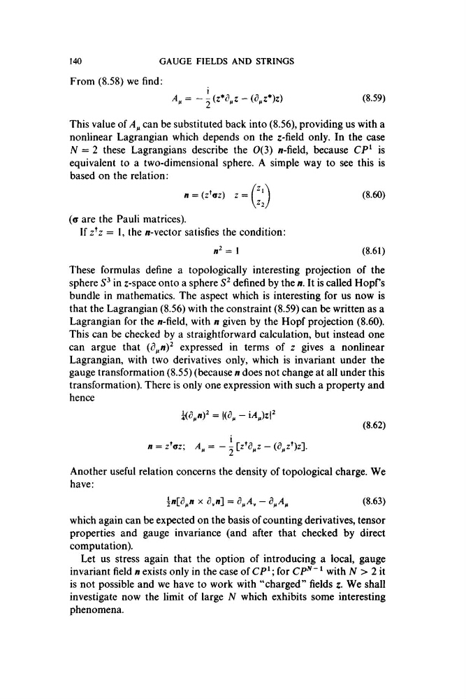
From (8.58) we find:
4^ = -
- (^^z*)z)
(8.59)
This value of can be substituted back into (8.56), providing us with a
nonlinear Lagrangian which depends on the ^-field only. In the case
N = 2 these Lagrangians describe the 0(3) /i-field, because CP^ is
equivalent to a two-dimensional sphere. A simple way to see this is
based on the relation:
n = (z^az)
(
n^ = \
(8.60)
(8.61)
These formulas define a topologically interesting projection of the
sphere in z-space onto a sphere defined by the n. It is called Hopf’s
bundle in mathematics. The aspect which is interesting for us now is
that the Lagrangian (8.56) with the constraint (8.59) can be written as a
Lagrangian for the «-field, with « given by the Hopf projection (8.60).
This can be checked by a straightforward calculation, but instead one
can argue that (d^ny expressed in terms of z gives a nonlinear
Lagrangian, with two derivatives only, which is invariant under the
gauge transformation (8.55) (because « does not change at all under this
transformation). There is only one expression with such a property and
hence
= \{d^ - iA^)zr
n =
A^ = - - Iz^d^z - (d^z^)z'].
(8.62)
Another useful relation concerns the density of topological charge. We
have:
\nld^ n X d,n ] = d^A,
(8.63)
which again can be expected on the basis of counting derivatives, tensor
properties and gauge invariance (and after that checked by direct
computation).
Let us stress again that the option of introducing a local, gauge
invariant field n exists only in the case of CP^; for CP^~^ with iV > 2 it
is not possible and we have to work with “charged” fields z. We shall
investigate now the limit of large N which exhibits some interesting
phenomena.
GAUGE FIELDS AND STRINGS
From (8.58) we find:
4^ = -
- (^^z*)z)
(8.59)
This value of can be substituted back into (8.56), providing us with a
nonlinear Lagrangian which depends on the ^-field only. In the case
N = 2 these Lagrangians describe the 0(3) /i-field, because CP^ is
equivalent to a two-dimensional sphere. A simple way to see this is
based on the relation:
n = (z^az)
(
n^ = \
(8.60)
(8.61)
These formulas define a topologically interesting projection of the
sphere in z-space onto a sphere defined by the n. It is called Hopf’s
bundle in mathematics. The aspect which is interesting for us now is
that the Lagrangian (8.56) with the constraint (8.59) can be written as a
Lagrangian for the «-field, with « given by the Hopf projection (8.60).
This can be checked by a straightforward calculation, but instead one
can argue that (d^ny expressed in terms of z gives a nonlinear
Lagrangian, with two derivatives only, which is invariant under the
gauge transformation (8.55) (because « does not change at all under this
transformation). There is only one expression with such a property and
hence
= \{d^ - iA^)zr
n =
A^ = - - Iz^d^z - (d^z^)z'].
(8.62)
Another useful relation concerns the density of topological charge. We
have:
\nld^ n X d,n ] = d^A,
(8.63)
which again can be expected on the basis of counting derivatives, tensor
properties and gauge invariance (and after that checked by direct
computation).
Let us stress again that the option of introducing a local, gauge
invariant field n exists only in the case of CP^; for CP^~^ with iV > 2 it
is not possible and we have to work with “charged” fields z. We shall
investigate now the limit of large N which exhibits some interesting
phenomena.