

THE LARGE N EXPANSION
1 37
We see, that because of the summation over c, the diagram in (8.46)
acquires a factor N which cancels the iV"Mn front.
It is easy to check that such a cancellation will take place in any
planar graph (i.e. a graph which does not have overlapping lines). For
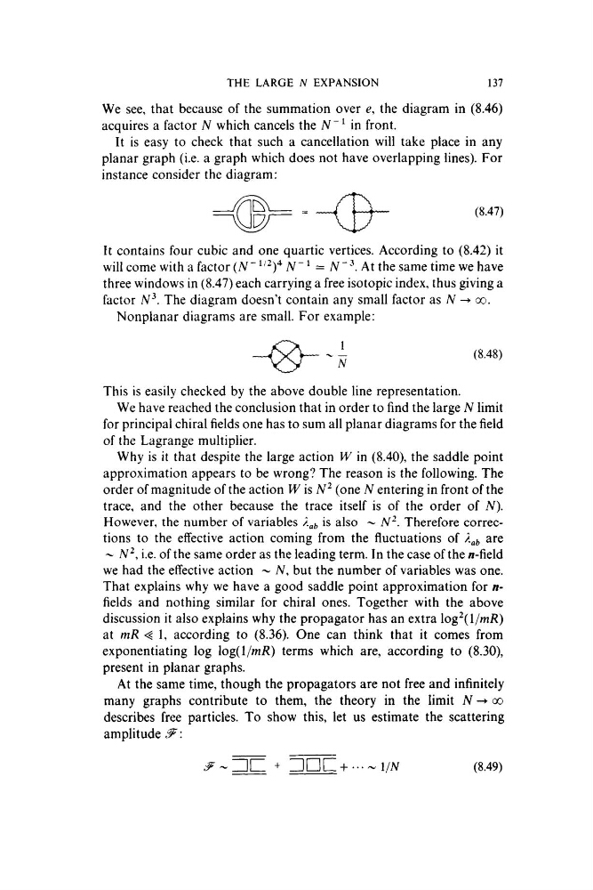
instance consider the diagram;
(8.47)
It contains four cubic and one quartic vertices. According to (8.42) it
will come with a factor (iV" ^^^)^
At the same time we have
three windows in (8.47) each carrying a free isotopic index, thus giving a
factor N^. The diagram doesn’t contain any small factor as jV -► oo.
Nonplanar diagrams are small. For example:
1
N
(8.48)
This is easily checked by the above double line representation.
We have reached the conclusion that in order to find the large N limit
for principal chiral fields one has to sum all planar diagrams for the field
of the Lagrange multiplier.
Why is it that despite the large action W in (8.40), the saddle point
approximation appears to be wrong? The reason is the following. The
order of magnitude of the action W is
(one N entering in front of the
trace, and the other because the trace itself is of the order of N).
However, the number of variables
is also ~
Therefore corrections to the effective action coming from the fluctuations of
are
^
i.e. of the same order as the leading term. In the case of the /i-field
we had the effective action ^ N, but the number of variables was one.
That explains why we have a good saddle point approximation for /ifields and nothing similar for chiral ones. Together with the above
discussion it also explains why the propagator has an extra \og^{\/mR)
at mR 1, according to (8.36). One can think that it comes from
exponentiating log \og{l/mR) terms which are, according to (8.30),
present in planar graphs.
At the same time, though the propagators are not free and infinitely
many graphs contribute to them, the theory in the limit N -► oo
describes free particles. To show this, let us estimate the scattering
amplitude 3^ :
\/N
(8.49)
1 37
We see, that because of the summation over c, the diagram in (8.46)
acquires a factor N which cancels the iV"Mn front.
It is easy to check that such a cancellation will take place in any
planar graph (i.e. a graph which does not have overlapping lines). For
instance consider the diagram;
(8.47)
It contains four cubic and one quartic vertices. According to (8.42) it
will come with a factor (iV" ^^^)^
At the same time we have
three windows in (8.47) each carrying a free isotopic index, thus giving a
factor N^. The diagram doesn’t contain any small factor as jV -► oo.
Nonplanar diagrams are small. For example:
1
N
(8.48)
This is easily checked by the above double line representation.
We have reached the conclusion that in order to find the large N limit
for principal chiral fields one has to sum all planar diagrams for the field
of the Lagrange multiplier.
Why is it that despite the large action W in (8.40), the saddle point
approximation appears to be wrong? The reason is the following. The
order of magnitude of the action W is
(one N entering in front of the
trace, and the other because the trace itself is of the order of N).
However, the number of variables
is also ~
Therefore corrections to the effective action coming from the fluctuations of
are
^
i.e. of the same order as the leading term. In the case of the /i-field
we had the effective action ^ N, but the number of variables was one.
That explains why we have a good saddle point approximation for /ifields and nothing similar for chiral ones. Together with the above
discussion it also explains why the propagator has an extra \og^{\/mR)
at mR 1, according to (8.36). One can think that it comes from
exponentiating log \og{l/mR) terms which are, according to (8.30),
present in planar graphs.
At the same time, though the propagators are not free and infinitely
many graphs contribute to them, the theory in the limit N -► oo
describes free particles. To show this, let us estimate the scattering
amplitude 3^ :
\/N
(8.49)