

128
GAUGE FIELDS AND STRINGS
explicitly how the strong coupling expansion connects without a phase
transition to the weak coupling region, giving (8.10).
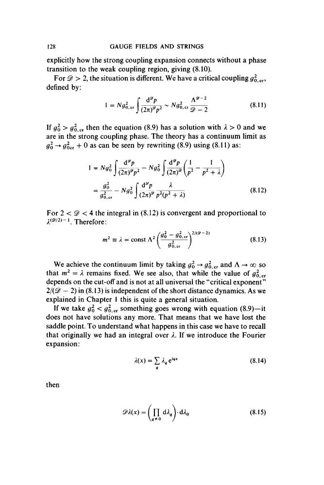
For ^ > 2, the situation is different. We have a critical coupling
defined by:
A^-2
(8.1 1 )
1 = Ngl,
d^p
{2nfp
' - 2
If gl > ^o,cr then the equation (8.9) has a solution with A > 0 and we
are in the strong coupling phase. The theory has a continuum limit as
gl -► ^ocr + 0 as can be seen by rewriting (8.9) using (8.11) as:
1 = % o (2nfp^
^0
2
i/o, cr
-
d®p
d®p / 1
(2nf VP‘
À
P À
(2nf p\p^ + X )
(8.12)
For 2 < ^ < 4 the integral in (8.12) is convergent and proportional to
^(^/2)-i xherefore:
w} = X = const A
/
\ 2/(^ 2)
2 / »0 ^0,c
do,C T /
(8.13)
We achieve the continuum limit by taking gl -► ^o,cr
A -> oo so
that
= X remains fixed. We see also, that while the value of ^o,cr
depends on the cut-off and is not at all universal the “critical exponent”
2/(^ — 2) in (8.13) is independent of the short distance dynamics. As we
explained in Chapter 1 this is quite a general situation.
If we take gl < g l something goes wrong with equation (8.9)—it
does not have solutions any more. That means that we have lost the
saddle point. To understand what happens in this case we have to recall
that originally we had an integral over X. If we introduce the Fourier
expansion:
A(x) =
(8.14)
then
^X{x) ■ ■ n
q^O
(8.15)
GAUGE FIELDS AND STRINGS
explicitly how the strong coupling expansion connects without a phase
transition to the weak coupling region, giving (8.10).
For ^ > 2, the situation is different. We have a critical coupling
defined by:
A^-2
(8.1 1 )
1 = Ngl,
d^p
{2nfp
' - 2
If gl > ^o,cr then the equation (8.9) has a solution with A > 0 and we
are in the strong coupling phase. The theory has a continuum limit as
gl -► ^ocr + 0 as can be seen by rewriting (8.9) using (8.11) as:
1 = % o (2nfp^
^0
2
i/o, cr
-
d®p
d®p / 1
(2nf VP‘
À
P À
(2nf p\p^ + X )
(8.12)
For 2 < ^ < 4 the integral in (8.12) is convergent and proportional to
^(^/2)-i xherefore:
w} = X = const A
/
\ 2/(^ 2)
2 / »0 ^0,c
do,C T /
(8.13)
We achieve the continuum limit by taking gl -► ^o,cr
A -> oo so
that
= X remains fixed. We see also, that while the value of ^o,cr
depends on the cut-off and is not at all universal the “critical exponent”
2/(^ — 2) in (8.13) is independent of the short distance dynamics. As we
explained in Chapter 1 this is quite a general situation.
If we take gl < g l something goes wrong with equation (8.9)—it
does not have solutions any more. That means that we have lost the
saddle point. To understand what happens in this case we have to recall
that originally we had an integral over X. If we introduce the Fourier
expansion:
A(x) =
(8.14)
then
^X{x) ■ ■ n
q^O
(8.15)