

ans=8×3 timetable
Time
velFun_EastWest
velFun_NorthSouth
velFun_Vertical
_________
_______________
_________________
_______________
8 sec
-0.56831
0.44642
1.8173
8.005 sec
-0.56831
0.45769
1.834
8.01 sec
-0.5786
0.46945
1.832
8.015 sec
-0.59869
0.48121
1.8114
8.02 sec
-0.62907
0.49346
1.7727
8.025 sec
-0.66925
0.5062
1.7154
8.03 sec
-0.71972
0.51894
1.6664
8.035 sec
-0.76088
0.53217
1.6257
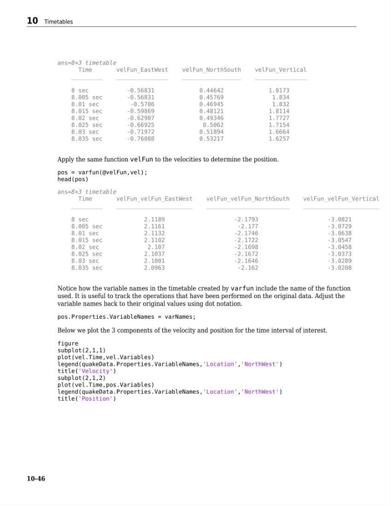
Apply the same function velFun to the velocities to determine the position.
pos = varfun(@velFun,vel);
head(pos)
ans=8×3 timetable
Time
velFun_velFun_EastWest
velFun_velFun_NorthSouth
velFun_velFun_Vertical
_________
______________________
________________________
______________________
8 sec
2.1189
-2.1793
-3.0821
8.005 sec
2.1161
-2.177
-3.0729
8.01 sec
2.1132
-2.1746
-3.0638
8.015 sec
2.1102
-2.1722
-3.0547
8.02 sec
2.107
-2.1698
-3.0458
8.025 sec
2.1037
-2.1672
-3.0373
8.03 sec
2.1001
-2.1646
-3.0289
8.035 sec
2.0963
-2.162
-3.0208
Notice how the variable names in the timetable created by varfun include the name of the function
used. It is useful to track the operations that have been performed on the original data. Adjust the
variable names back to their original values using dot notation.
pos.Properties.VariableNames = varNames;
Below we plot the 3 components of the velocity and position for the time interval of interest.
figure
subplot(2,1,1)
plot(vel.Time,vel.Variables)
legend(quakeData.Properties.VariableNames,'Location','NorthWest')
title('Velocity')
subplot(2,1,2)
plot(vel.Time,pos.Variables)
legend(quakeData.Properties.VariableNames,'Location','NorthWest')
title('Position')
10 Timetables
10-46
Time
velFun_EastWest
velFun_NorthSouth
velFun_Vertical
_________
_______________
_________________
_______________
8 sec
-0.56831
0.44642
1.8173
8.005 sec
-0.56831
0.45769
1.834
8.01 sec
-0.5786
0.46945
1.832
8.015 sec
-0.59869
0.48121
1.8114
8.02 sec
-0.62907
0.49346
1.7727
8.025 sec
-0.66925
0.5062
1.7154
8.03 sec
-0.71972
0.51894
1.6664
8.035 sec
-0.76088
0.53217
1.6257
Apply the same function velFun to the velocities to determine the position.
pos = varfun(@velFun,vel);
head(pos)
ans=8×3 timetable
Time
velFun_velFun_EastWest
velFun_velFun_NorthSouth
velFun_velFun_Vertical
_________
______________________
________________________
______________________
8 sec
2.1189
-2.1793
-3.0821
8.005 sec
2.1161
-2.177
-3.0729
8.01 sec
2.1132
-2.1746
-3.0638
8.015 sec
2.1102
-2.1722
-3.0547
8.02 sec
2.107
-2.1698
-3.0458
8.025 sec
2.1037
-2.1672
-3.0373
8.03 sec
2.1001
-2.1646
-3.0289
8.035 sec
2.0963
-2.162
-3.0208
Notice how the variable names in the timetable created by varfun include the name of the function
used. It is useful to track the operations that have been performed on the original data. Adjust the
variable names back to their original values using dot notation.
pos.Properties.VariableNames = varNames;
Below we plot the 3 components of the velocity and position for the time interval of interest.
figure
subplot(2,1,1)
plot(vel.Time,vel.Variables)
legend(quakeData.Properties.VariableNames,'Location','NorthWest')
title('Velocity')
subplot(2,1,2)
plot(vel.Time,pos.Variables)
legend(quakeData.Properties.VariableNames,'Location','NorthWest')
title('Position')
10 Timetables
10-46