

Chapter 8
Maclaurin’s series
8.1 Introduction
Some mathematical functions may be represented as
power series, containing terms in ascending powers of
the variable. For example,
e
x
= 1 + x +
x 2
2!
+
x 3
3!
+ · · ·
sin x = x −
x 3
3!
+
x 5
5!
−
x 7
7!
+ · · ·
and cosh x = 1 +
x 2
2!
+
x 4
4!
+ · · ·
(as introduced in Chapter 5)
Using a series, called Maclaurin’s series, mixed functions containing, say, algebraic, trigonometric and exponential functions, may be expressed solely as algebraic
functions, and differentiation and integration can often
be more readily performed.
To expand a function using Maclaurin’s theorem,
some knowledge of differentiation is needed (More on
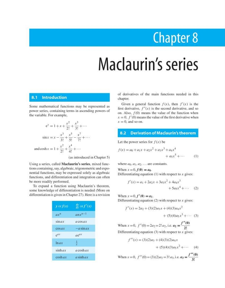
differentiation is given in Chapter 27). Here is a revision
y or f(x)
dy
dx or f
(x)
ax n
anx n−1
sin ax
a cos ax
cos ax
−a sin ax
e ax
ae ax
ln ax
1
x
sinh ax
a cosh ax
cosh ax
a sinh ax
of derivatives of the main functions needed in this
chapter.
Given a general function f (x), then f (x) is the
first derivative, f (x) is the second derivative, and so
on. Also, f (0) means the value of the function when
x = 0, f (0) means the value of the first derivative when
x = 0, and so on.
8.2 Derivation of Maclaurin’s theorem
Let the power series for f (x) be
f (x) = a 0 + a 1 x + a 2 x
2
+ a 3 x
3
+ a 4 x
4
+ a 5 x
5
+ · · ·
(1)
where a 0 , a 1 , a 2 , ... are constants.
When x = 0, f(0) = a 0 .
Differentiating equation (1) with respect to x gives:
f
(x) = a 1 + 2a 2 x + 3a 3 x
2
+ 4a 4 x
3
+ 5a 5 x
4
+ · · · (2)
When x = 0, f (0) = a 1 .
Differentiating equation (2) with respect to x gives:
f
(x) = 2a 2 + (3)(2)a 3 x + (4)(3)a 4 x
2
+ (5)(4)a 5 x
3
+ · · · (3)
When x = 0, f (0) = 2a 2 = 2! a 2 , i.e. a 2 =
f
(0)
2!
Differentiating equation (3) with respect to x gives:
f
(x) = (3)(2)a 3 + (4)(3)(2)a 4 x
+ (5)(4)(3)a 5 x
2
+ · · ·
(4)
When x = 0, f (0) = (3)(2)a 3 = 3! a 3 , i.e. a 3 =
f
(0)
3!
Maclaurin’s series
8.1 Introduction
Some mathematical functions may be represented as
power series, containing terms in ascending powers of
the variable. For example,
e
x
= 1 + x +
x 2
2!
+
x 3
3!
+ · · ·
sin x = x −
x 3
3!
+
x 5
5!
−
x 7
7!
+ · · ·
and cosh x = 1 +
x 2
2!
+
x 4
4!
+ · · ·
(as introduced in Chapter 5)
Using a series, called Maclaurin’s series, mixed functions containing, say, algebraic, trigonometric and exponential functions, may be expressed solely as algebraic
functions, and differentiation and integration can often
be more readily performed.
To expand a function using Maclaurin’s theorem,
some knowledge of differentiation is needed (More on
differentiation is given in Chapter 27). Here is a revision
y or f(x)
dy
dx or f
(x)
ax n
anx n−1
sin ax
a cos ax
cos ax
−a sin ax
e ax
ae ax
ln ax
1
x
sinh ax
a cosh ax
cosh ax
a sinh ax
of derivatives of the main functions needed in this
chapter.
Given a general function f (x), then f (x) is the
first derivative, f (x) is the second derivative, and so
on. Also, f (0) means the value of the function when
x = 0, f (0) means the value of the first derivative when
x = 0, and so on.
8.2 Derivation of Maclaurin’s theorem
Let the power series for f (x) be
f (x) = a 0 + a 1 x + a 2 x
2
+ a 3 x
3
+ a 4 x
4
+ a 5 x
5
+ · · ·
(1)
where a 0 , a 1 , a 2 , ... are constants.
When x = 0, f(0) = a 0 .
Differentiating equation (1) with respect to x gives:
f
(x) = a 1 + 2a 2 x + 3a 3 x
2
+ 4a 4 x
3
+ 5a 5 x
4
+ · · · (2)
When x = 0, f (0) = a 1 .
Differentiating equation (2) with respect to x gives:
f
(x) = 2a 2 + (3)(2)a 3 x + (4)(3)a 4 x
2
+ (5)(4)a 5 x
3
+ · · · (3)
When x = 0, f (0) = 2a 2 = 2! a 2 , i.e. a 2 =
f
(0)
2!
Differentiating equation (3) with respect to x gives:
f
(x) = (3)(2)a 3 + (4)(3)(2)a 4 x
+ (5)(4)(3)a 5 x
2
+ · · ·
(4)
When x = 0, f (0) = (3)(2)a 3 = 3! a 3 , i.e. a 3 =
f
(0)
3!