

612 Higher Engineering Mathematics
f (x) = a 0 +
∞
n=1
(a n cos nx + b n sinnx) (1)
where for the range −π to π:
and
a 0 =
1
2π
π
−π
f (x) dx
a n =
1
π
π
−π
f (x)cos nx dx
(n = 1, 2, 3, . ..)
b n =
1
π
π
−π
f (x)sin nx dx
(n = 1, 2, 3, . ..)
(ii) a 0 , a n and b n are called the Fourier coefficients
of the series and if these can be determined, the
series of equation (1) is called the Fourier series
corresponding to f (x).
(iii) An alternative way of writing the series is by
using the a cos x + b sin x = c sin(x + α) relationship introduced in Chapter 17, i.e.
f (x) = a 0 + c 1 sin(x + α 1 ) + c 2 sin(2x + α 2 )
+ · · · + c n sin(nx + α n ),
where a 0 is a constant,
c 1 =
(a
2
1 + b
2
1 ), ...c n =
(a 2
n + b 2
n )
are the amplitudes of the various components,
and phase angle
α n = tan
−1 a n
b n
(iv) For the series of equation (1): the term
(a 1 cos x + b 1 sin x) or c 1 sin(x + α 1 ) is called the
first harmonic or the fundamental, the term
(a 2 cos 2x + b 2 sin 2x) or c 2 sin(2x + α 2 ) is called
the second harmonic, and so on.
For an exact representation of a complex wave, an infinite number of terms are, in general, required. In many
practical cases, however, it is sufficient to take the first
few terms only (see Problem 2).
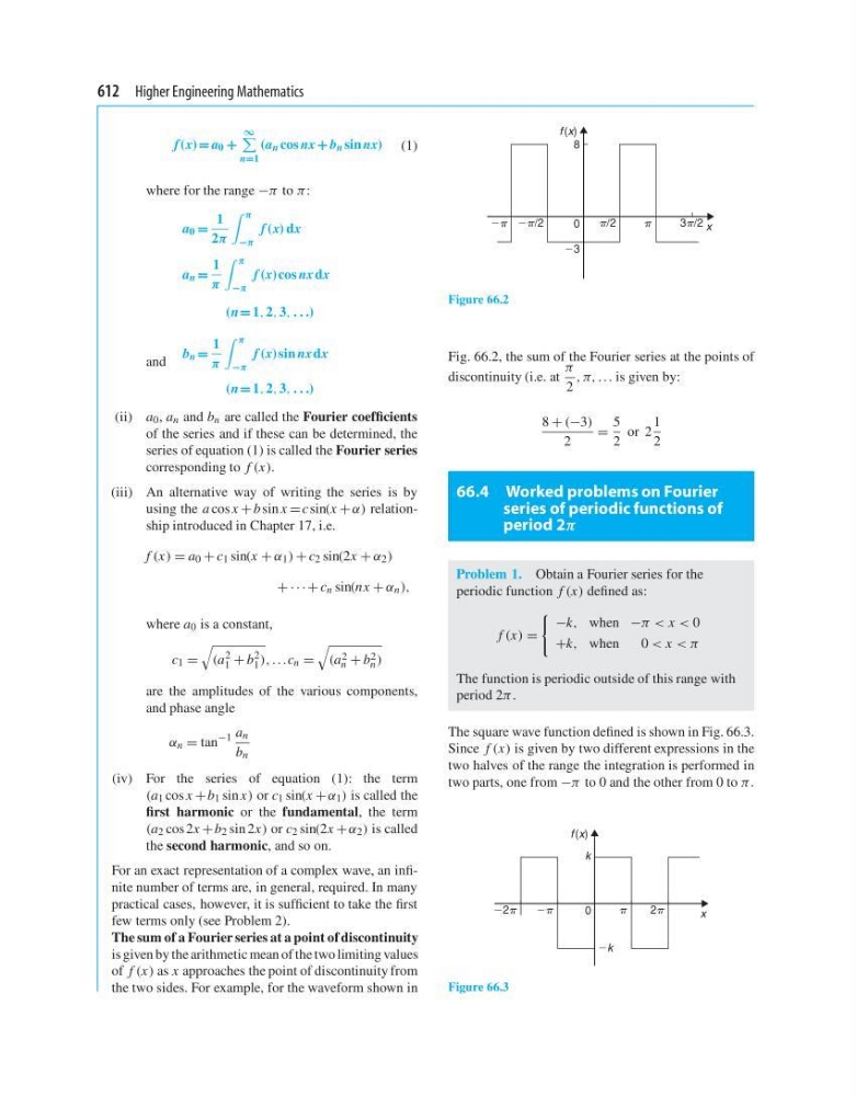
The sum of a Fourier series at a point of discontinuity
is given by the arithmetic mean of the two limiting values
of f (x) as x approaches the point of discontinuity from
the two sides. For example, for the waveform shown in
x
f (x)
3/2
0
8
23
2/2
/2
2
Figure 66.2
Fig. 66.2, the sum of the Fourier series at the points of
discontinuity (i.e. at
π
2
, π, ... is given by:
8 + (−3)
2
=
5
2
or 2
1
2
66.4 Worked problems on Fourier
series of periodic functions of
period 2π
Problem 1. Obtain a Fourier series for the
periodic function f (x) defined as:
f (x) =
−k, when −π < x < 0
+k, when
0 < x < π
The function is periodic outside of this range with
period 2π.
The square wave function defined is shown in Fig. 66.3.
Since f (x) is given by two different expressions in the
two halves of the range the integration is performed in
two parts, one from −π to 0 and the other from 0 to π.
x
f (x)
2
0
k
2k
22
2
Figure 66.3
f (x) = a 0 +
∞
n=1
(a n cos nx + b n sinnx) (1)
where for the range −π to π:
and
a 0 =
1
2π
π
−π
f (x) dx
a n =
1
π
π
−π
f (x)cos nx dx
(n = 1, 2, 3, . ..)
b n =
1
π
π
−π
f (x)sin nx dx
(n = 1, 2, 3, . ..)
(ii) a 0 , a n and b n are called the Fourier coefficients
of the series and if these can be determined, the
series of equation (1) is called the Fourier series
corresponding to f (x).
(iii) An alternative way of writing the series is by
using the a cos x + b sin x = c sin(x + α) relationship introduced in Chapter 17, i.e.
f (x) = a 0 + c 1 sin(x + α 1 ) + c 2 sin(2x + α 2 )
+ · · · + c n sin(nx + α n ),
where a 0 is a constant,
c 1 =
(a
2
1 + b
2
1 ), ...c n =
(a 2
n + b 2
n )
are the amplitudes of the various components,
and phase angle
α n = tan
−1 a n
b n
(iv) For the series of equation (1): the term
(a 1 cos x + b 1 sin x) or c 1 sin(x + α 1 ) is called the
first harmonic or the fundamental, the term
(a 2 cos 2x + b 2 sin 2x) or c 2 sin(2x + α 2 ) is called
the second harmonic, and so on.
For an exact representation of a complex wave, an infinite number of terms are, in general, required. In many
practical cases, however, it is sufficient to take the first
few terms only (see Problem 2).
The sum of a Fourier series at a point of discontinuity
is given by the arithmetic mean of the two limiting values
of f (x) as x approaches the point of discontinuity from
the two sides. For example, for the waveform shown in
x
f (x)
3/2
0
8
23
2/2
/2
2
Figure 66.2
Fig. 66.2, the sum of the Fourier series at the points of
discontinuity (i.e. at
π
2
, π, ... is given by:
8 + (−3)
2
=
5
2
or 2
1
2
66.4 Worked problems on Fourier
series of periodic functions of
period 2π
Problem 1. Obtain a Fourier series for the
periodic function f (x) defined as:
f (x) =
−k, when −π < x < 0
+k, when
0 < x < π
The function is periodic outside of this range with
period 2π.
The square wave function defined is shown in Fig. 66.3.
Since f (x) is given by two different expressions in the
two halves of the range the integration is performed in
two parts, one from −π to 0 and the other from 0 to π.
x
f (x)
2
0
k
2k
22
2
Figure 66.3