

598 Higher Engineering Mathematics
7.
26 −s 2
s(s 2 + 4s + 13)
2 − 3e −2t cos 3t −
2
3
e −2t sin 3t
63.4 Poles and zeros
It was seen in the previous section that Laplace transforms, in general, have the form f (s) =
φ(s)
θ(s)
. This is
the same form as most transfer functions for engineering systems, a transfer function being one that relates
the response at a given pair of terminals to a source or
stimulus at another pair of terminals.
Let a function in the s domain be given by:
f (s) =
φ(s)
(s − a)(s − b)(s − c)
where φ(s) is of less
degree than the denominator.
Poles: The values a, b, c, … that makes the denominator zero, and hence f (s) infinite, are called
the system poles of f (s).
If there are no repeated factors, the poles are
simple poles.
If there are repeated factors, the poles are
multiple poles.
Zeros: Values of s that make the numerator φ(s) zero,
and hence f (s) zero, are called the system
zeros of f (s).
For example:
s − 4
(s + 1)(s − 2)
has simple poles at s =−1
and s =+2, and a zero at s = 4
s + 3
(s + 1) 2 (2s + 5)
has a
simple pole at s =−
5
2
and double poles at s =−1, and
a zero at s = −3 and
s + 2
s(s − 1)(s + 4)(2s + 1)
has simple
poles at s = 0, +1, −4, and −
1
2
and a zero at s =−2
Pole-zero diagram
The poles and zeros of a function are values of complex
frequency s and can therefore be plotted on the complex
frequency or s-plane. The resulting plot is the pole-zero
diagram or pole-zero map. On the rectangular axes, the
real part is labelled the σ -axis and the imaginary part
the jω-axis.
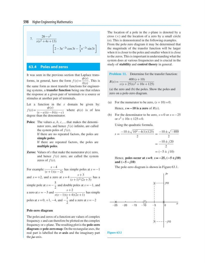
The location of a pole in the s-plane is denoted by a
cross (×) and the location of a zero by a small circle
(o). This is demonstrated in the following examples.
From the pole-zero diagram it may be determined that
the magnitude of the transfer function will be larger
when it is closer to the poles and smaller when it is close
to the zeros. This is important in understanding what the
system does at various frequencies and is crucial in the
study of stability and control theory in general.
Problem 11. Determine for the transfer function:
R(s) =
400 (s + 10)
s (s + 25)(s 2 + 10s + 125)
(a) the zero and (b) the poles. Show the poles and
zero on a pole-zero diagram.
(a) For the numerator to be zero, (s + 10) = 0.
Hence, s =−10 is a zero of R(s).
(b) For the denominator to be zero, s = 0 or s =−25
or s 2 + 10s + 125 =0.
Using the quadratic formula.
s =
−10 ±
10 2 −4(1)(125)
2
=
−10 ±
√
−400
2
=
−10 ± j 20
2
= (−5 ± j 10)
Hence, poles occur at s = 0, s =−25, (−5 + j10)
and (−5 −j10)
The pole-zero diagram is shown in Figure 63.1.
210
0
2j10
j10
j
215
220
225
25
Figure 63.1
7.
26 −s 2
s(s 2 + 4s + 13)
2 − 3e −2t cos 3t −
2
3
e −2t sin 3t
63.4 Poles and zeros
It was seen in the previous section that Laplace transforms, in general, have the form f (s) =
φ(s)
θ(s)
. This is
the same form as most transfer functions for engineering systems, a transfer function being one that relates
the response at a given pair of terminals to a source or
stimulus at another pair of terminals.
Let a function in the s domain be given by:
f (s) =
φ(s)
(s − a)(s − b)(s − c)
where φ(s) is of less
degree than the denominator.
Poles: The values a, b, c, … that makes the denominator zero, and hence f (s) infinite, are called
the system poles of f (s).
If there are no repeated factors, the poles are
simple poles.
If there are repeated factors, the poles are
multiple poles.
Zeros: Values of s that make the numerator φ(s) zero,
and hence f (s) zero, are called the system
zeros of f (s).
For example:
s − 4
(s + 1)(s − 2)
has simple poles at s =−1
and s =+2, and a zero at s = 4
s + 3
(s + 1) 2 (2s + 5)
has a
simple pole at s =−
5
2
and double poles at s =−1, and
a zero at s = −3 and
s + 2
s(s − 1)(s + 4)(2s + 1)
has simple
poles at s = 0, +1, −4, and −
1
2
and a zero at s =−2
Pole-zero diagram
The poles and zeros of a function are values of complex
frequency s and can therefore be plotted on the complex
frequency or s-plane. The resulting plot is the pole-zero
diagram or pole-zero map. On the rectangular axes, the
real part is labelled the σ -axis and the imaginary part
the jω-axis.
The location of a pole in the s-plane is denoted by a
cross (×) and the location of a zero by a small circle
(o). This is demonstrated in the following examples.
From the pole-zero diagram it may be determined that
the magnitude of the transfer function will be larger
when it is closer to the poles and smaller when it is close
to the zeros. This is important in understanding what the
system does at various frequencies and is crucial in the
study of stability and control theory in general.
Problem 11. Determine for the transfer function:
R(s) =
400 (s + 10)
s (s + 25)(s 2 + 10s + 125)
(a) the zero and (b) the poles. Show the poles and
zero on a pole-zero diagram.
(a) For the numerator to be zero, (s + 10) = 0.
Hence, s =−10 is a zero of R(s).
(b) For the denominator to be zero, s = 0 or s =−25
or s 2 + 10s + 125 =0.
Using the quadratic formula.
s =
−10 ±
10 2 −4(1)(125)
2
=
−10 ±
√
−400
2
=
−10 ± j 20
2
= (−5 ± j 10)
Hence, poles occur at s = 0, s =−25, (−5 + j10)
and (−5 −j10)
The pole-zero diagram is shown in Figure 63.1.
210
0
2j10
j10
j
215
220
225
25
Figure 63.1