

576 Higher Engineering Mathematics
in Fig. 60.1 and the co-ordinate values (H 3 , H 4 , etc.)
are taken as the deviations. The equation of the regression line is of the form: X =b 0 + b 1 Y and the normal
equations become:
X = b 0 N + b 1
Y
(3)
(XY) = b 0
Y + b 1
Y
2
(4)
where X and Y are the co-ordinate values, b 0 and b 1
are the regression coefficients of X on Y and N is the
number of co-ordinates. These normal equations are of
the regression line of X on Y , which is slightly different
to the regression line of Y on X . The regression line of
X on Y is used to estimated values of X for given values
of Y . The regression line of Y on X is used to determine
any value of Y corresponding to a given value of X . If
the value of Y lies within the range of Y -values of the
extreme co-ordinates, the process of finding the corresponding value of X is called linear interpolation. If
it lies outside of the range of Y -values of the extreme
co-ordinates than the process is called linear extrapolation and the assumption must be made that the line of
best fit extends outside of the range of the co-ordinate
values given.
By using the regression line of X on Y , values of X
corresponding to given values of Y may be found by
either interpolation or extrapolation.
60.3 Worked problems on linear
regression
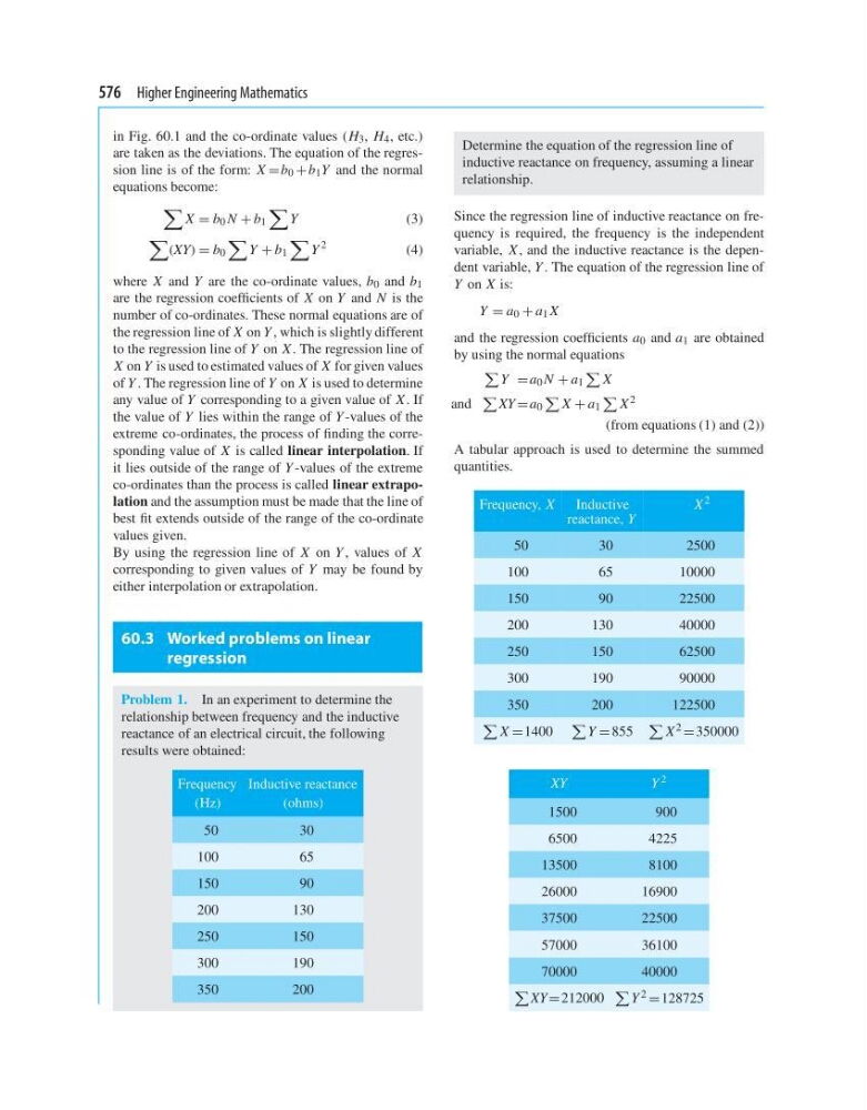
Problem 1. In an experiment to determine the
relationship between frequency and the inductive
reactance of an electrical circuit, the following
results were obtained:
Frequency Inductive reactance
(Hz)
(ohms)
50
30
100
65
150
90
200
130
250
150
300
190
350
200
Determine the equation of the regression line of
inductive reactance on frequency, assuming a linear
relationship.
Since the regression line of inductive reactance on frequency is required, the frequency is the independent
variable, X , and the inductive reactance is the dependent variable, Y . The equation of the regression line of
Y on X is:
Y = a 0 + a 1 X
and the regression coefficients a 0 and a 1 are obtained
by using the normal equations
Y = a 0 N + a 1
X
and
XY = a 0
X + a 1
X 2
(from equations (1) and (2))
A tabular approach is used to determine the summed
quantities.
Frequency, X
Inductive
X 2
reactance, Y
50
30
2500
100
65
10000
150
90
22500
200
130
40000
250
150
62500
300
190
90000
350
200
122500
X =1400
Y = 855
X 2 = 350000
XY
Y 2
1500
900
6500
4225
13500
8100
26000
16900
37500
22500
57000
36100
70000
40000
XY = 212000
Y 2 = 128725
in Fig. 60.1 and the co-ordinate values (H 3 , H 4 , etc.)
are taken as the deviations. The equation of the regression line is of the form: X =b 0 + b 1 Y and the normal
equations become:
X = b 0 N + b 1
Y
(3)
(XY) = b 0
Y + b 1
Y
2
(4)
where X and Y are the co-ordinate values, b 0 and b 1
are the regression coefficients of X on Y and N is the
number of co-ordinates. These normal equations are of
the regression line of X on Y , which is slightly different
to the regression line of Y on X . The regression line of
X on Y is used to estimated values of X for given values
of Y . The regression line of Y on X is used to determine
any value of Y corresponding to a given value of X . If
the value of Y lies within the range of Y -values of the
extreme co-ordinates, the process of finding the corresponding value of X is called linear interpolation. If
it lies outside of the range of Y -values of the extreme
co-ordinates than the process is called linear extrapolation and the assumption must be made that the line of
best fit extends outside of the range of the co-ordinate
values given.
By using the regression line of X on Y , values of X
corresponding to given values of Y may be found by
either interpolation or extrapolation.
60.3 Worked problems on linear
regression
Problem 1. In an experiment to determine the
relationship between frequency and the inductive
reactance of an electrical circuit, the following
results were obtained:
Frequency Inductive reactance
(Hz)
(ohms)
50
30
100
65
150
90
200
130
250
150
300
190
350
200
Determine the equation of the regression line of
inductive reactance on frequency, assuming a linear
relationship.
Since the regression line of inductive reactance on frequency is required, the frequency is the independent
variable, X , and the inductive reactance is the dependent variable, Y . The equation of the regression line of
Y on X is:
Y = a 0 + a 1 X
and the regression coefficients a 0 and a 1 are obtained
by using the normal equations
Y = a 0 N + a 1
X
and
XY = a 0
X + a 1
X 2
(from equations (1) and (2))
A tabular approach is used to determine the summed
quantities.
Frequency, X
Inductive
X 2
reactance, Y
50
30
2500
100
65
10000
150
90
22500
200
130
40000
250
150
62500
300
190
90000
350
200
122500
X =1400
Y = 855
X 2 = 350000
XY
Y 2
1500
900
6500
4225
13500
8100
26000
16900
37500
22500
57000
36100
70000
40000
XY = 212000
Y 2 = 128725