

Chapter 60
Linear regression
60.1 Introduction to linear regression
Regression analysis, usually termed regression, is used
to draw the line of ‘best fit’ through co-ordinates on
a graph. The techniques used enable a mathematical equation of the straight line form y = mx + c to
be deduced for a given set of co-ordinate values, the
line being such that the sum of the deviations of
the co-ordinate values from the line is a minimum,
i.e. it is the line of ‘best fit’. When a regression analysis is made, it is possible to obtain two lines of best fit,
depending on which variable is selected as the dependent variable and which variable is the independent
variable. For example, in a resistive electrical circuit, the
current flowing is directly proportional to the voltage
applied to the circuit. There are two ways of obtaining experimental values relating the current and voltage.
Either, certain voltages are applied to the circuit and the
current values are measured, in which case the voltage is
the independent variable and the current is the dependent
variable; or, the voltage can be adjusted until a desired
value of current is flowing and the value of voltage is
measured, in which case the current is the independent
value and the voltage is the dependent value.
60.2 The least-squares regression
lines
For a given set of co-ordinate values, (X 1 , Y 1 ),
(X 2 , Y 2 ), ..., (X n , Y n ) let the X values be the independent variables and the Y -values be the dependent values.
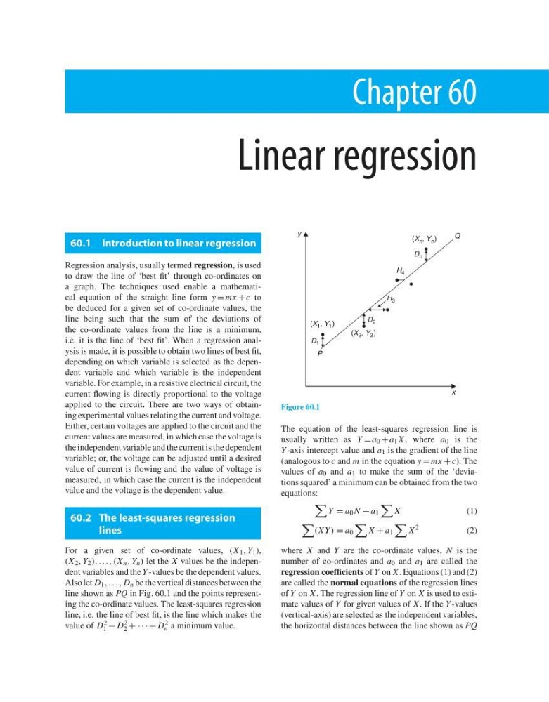
Also let D 1 , ..., D n be the vertical distances between the
line shown as PQ in Fig. 60.1 and the points representing the co-ordinate values. The least-squares regression
line, i.e. the line of best fit, is the line which makes the
value of D 2
1 + D 2
2 + · · · + D 2
n a minimum value.
x
y
Q
(X 1 , Y 1 )
(X 2 , Y 2 )
(X n , Y n )
D 1
D 2
D n
H 3
H 4
P
Figure 60.1
The equation of the least-squares regression line is
usually written as Y = a 0 + a 1 X , where a 0 is the
Y -axis intercept value and a 1 is the gradient of the line
(analogous to c and m in the equation y = mx + c). The
values of a 0 and a 1 to make the sum of the ‘deviations squared’ a minimum can be obtained from the two
equations:
Y = a 0 N + a 1
X
(1)
(X Y ) = a 0
X + a 1
X
2
(2)
where X and Y are the co-ordinate values, N is the
number of co-ordinates and a 0 and a 1 are called the
regression coefficients of Y on X . Equations (1) and (2)
are called the normal equations of the regression lines
of Y on X . The regression line of Y on X is used to estimate values of Y for given values of X . If the Y -values
(vertical-axis) are selected as the independent variables,
the horizontal distances between the line shown as PQ
Linear regression
60.1 Introduction to linear regression
Regression analysis, usually termed regression, is used
to draw the line of ‘best fit’ through co-ordinates on
a graph. The techniques used enable a mathematical equation of the straight line form y = mx + c to
be deduced for a given set of co-ordinate values, the
line being such that the sum of the deviations of
the co-ordinate values from the line is a minimum,
i.e. it is the line of ‘best fit’. When a regression analysis is made, it is possible to obtain two lines of best fit,
depending on which variable is selected as the dependent variable and which variable is the independent
variable. For example, in a resistive electrical circuit, the
current flowing is directly proportional to the voltage
applied to the circuit. There are two ways of obtaining experimental values relating the current and voltage.
Either, certain voltages are applied to the circuit and the
current values are measured, in which case the voltage is
the independent variable and the current is the dependent
variable; or, the voltage can be adjusted until a desired
value of current is flowing and the value of voltage is
measured, in which case the current is the independent
value and the voltage is the dependent value.
60.2 The least-squares regression
lines
For a given set of co-ordinate values, (X 1 , Y 1 ),
(X 2 , Y 2 ), ..., (X n , Y n ) let the X values be the independent variables and the Y -values be the dependent values.
Also let D 1 , ..., D n be the vertical distances between the
line shown as PQ in Fig. 60.1 and the points representing the co-ordinate values. The least-squares regression
line, i.e. the line of best fit, is the line which makes the
value of D 2
1 + D 2
2 + · · · + D 2
n a minimum value.
x
y
Q
(X 1 , Y 1 )
(X 2 , Y 2 )
(X n , Y n )
D 1
D 2
D n
H 3
H 4
P
Figure 60.1
The equation of the least-squares regression line is
usually written as Y = a 0 + a 1 X , where a 0 is the
Y -axis intercept value and a 1 is the gradient of the line
(analogous to c and m in the equation y = mx + c). The
values of a 0 and a 1 to make the sum of the ‘deviations squared’ a minimum can be obtained from the two
equations:
Y = a 0 N + a 1
X
(1)
(X Y ) = a 0
X + a 1
X
2
(2)
where X and Y are the co-ordinate values, N is the
number of co-ordinates and a 0 and a 1 are called the
regression coefficients of Y on X . Equations (1) and (2)
are called the normal equations of the regression lines
of Y on X . The regression line of Y on X is used to estimate values of Y for given values of X . If the Y -values
(vertical-axis) are selected as the independent variables,
the horizontal distances between the line shown as PQ