

An introduction to partial differential equations 525
=
30
nπ
(1 − cos nπ)
= 0 (when n is even) and
60
nπ
(when n is odd)
Hence, the required solution is:
u(x, t) =
∞
n=1
Q n e
− p 2 c 2 t sin nπ x
=
60
π
∞
n(odd)=1
1
n
(sin nπ x)e
−n 2 π 2 c 2 t
Now try the following exercise
Exercise 202 Further problems on the heat
conduction equation
1. A metal bar, insulated along its sides, is 4 m
long. It is initially at a temperature of 10 ◦ C
and at time t = 0, the ends are placed into ice at
0 ◦ C. Find an expression for the temperature
at a point P at a distance x m from one end at
any time t seconds after t = 0.
⎡
⎣ u(x, t ) =
40
π
∞
n(odd)=1
1
n
e
−
n 2 π 2 c 2 t
16
sin
nπ x
4
⎤
⎦
2. An insulated uniform metal bar, 8 m long,
has the temperature of its ends maintained at
0 ◦ C, and at time t = 0 the temperature distribution f (x) along the bar is defined by
f (x) = x(8 − x). If c
2
= 1, solve the heat conduction equation
∂ 2 u
∂x 2 =
1
c 2
∂u
∂t
to determine
the temperature u at any point in the bar at
time t .
⎡
⎣ u(x, t ) =
8
π
3 ∞
n(odd)=1
1
n 3 e
−
n 2 π 2 t
64 sin
nπ x
8
⎤
⎦
3. The ends of an insulated rod PQ, 20 units long,
are maintained at 0
◦ C. At time t = 0, the temperature within the rod rises uniformly from
each end reaching 4 ◦ C at the mid-point of
PQ. Find an expression for the temperature
u(x, t ) at any point in the rod, distant x from
P at any time t after t = 0. Assume the heat
conduction equation to be
∂ 2 u
∂x 2 =
1
c 2
∂u
∂t
and
take c 2 = 1.
⎡
⎣ u(x, t ) =
320
π 2
∞
n(odd)=1
1
n 2 sin
nπ
2
sin
nπ x
20
e
−
n 2 π 2 t
400
⎤
⎦
53.8 Laplace’s equation
The distribution of electrical potential, or temperature,
over a plane area subject to certain boundary conditions,
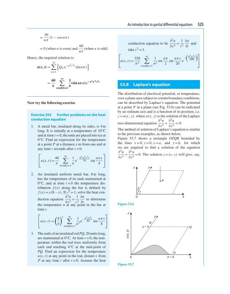
can be described by Laplace’s equation. The potential
at a point P in a plane (see Fig. 53.6) can be indicated
by an ordinate axis and is a function of its position, i.e.
z = u(x, y), where u(x, y) is the solution of the Laplace
two-dimensional equation
∂
2 u
∂x 2 +
∂
2 u
∂ y 2 = 0.
The method of solution of Laplace’s equation is similar
to the previous examples, as shown below.
Figure 53.7 shows a rectangle OPQR bounded by
the lines x = 0, y = 0, x = a, and y = b, for which
we are required to find a solution of the equation
∂ 2 u
∂x 2 +
∂ 2 u
∂ y 2 = 0. The solution z =(x, y) will give, say,
0
x
z
y
P
Figure 53.6
0
x
z
y
u (x, y )
P
Q
R
y 5 b
x 5 a
Figure 53.7
=
30
nπ
(1 − cos nπ)
= 0 (when n is even) and
60
nπ
(when n is odd)
Hence, the required solution is:
u(x, t) =
∞
n=1
Q n e
− p 2 c 2 t sin nπ x
=
60
π
∞
n(odd)=1
1
n
(sin nπ x)e
−n 2 π 2 c 2 t
Now try the following exercise
Exercise 202 Further problems on the heat
conduction equation
1. A metal bar, insulated along its sides, is 4 m
long. It is initially at a temperature of 10 ◦ C
and at time t = 0, the ends are placed into ice at
0 ◦ C. Find an expression for the temperature
at a point P at a distance x m from one end at
any time t seconds after t = 0.
⎡
⎣ u(x, t ) =
40
π
∞
n(odd)=1
1
n
e
−
n 2 π 2 c 2 t
16
sin
nπ x
4
⎤
⎦
2. An insulated uniform metal bar, 8 m long,
has the temperature of its ends maintained at
0 ◦ C, and at time t = 0 the temperature distribution f (x) along the bar is defined by
f (x) = x(8 − x). If c
2
= 1, solve the heat conduction equation
∂ 2 u
∂x 2 =
1
c 2
∂u
∂t
to determine
the temperature u at any point in the bar at
time t .
⎡
⎣ u(x, t ) =
8
π
3 ∞
n(odd)=1
1
n 3 e
−
n 2 π 2 t
64 sin
nπ x
8
⎤
⎦
3. The ends of an insulated rod PQ, 20 units long,
are maintained at 0
◦ C. At time t = 0, the temperature within the rod rises uniformly from
each end reaching 4 ◦ C at the mid-point of
PQ. Find an expression for the temperature
u(x, t ) at any point in the rod, distant x from
P at any time t after t = 0. Assume the heat
conduction equation to be
∂ 2 u
∂x 2 =
1
c 2
∂u
∂t
and
take c 2 = 1.
⎡
⎣ u(x, t ) =
320
π 2
∞
n(odd)=1
1
n 2 sin
nπ
2
sin
nπ x
20
e
−
n 2 π 2 t
400
⎤
⎦
53.8 Laplace’s equation
The distribution of electrical potential, or temperature,
over a plane area subject to certain boundary conditions,
can be described by Laplace’s equation. The potential
at a point P in a plane (see Fig. 53.6) can be indicated
by an ordinate axis and is a function of its position, i.e.
z = u(x, y), where u(x, y) is the solution of the Laplace
two-dimensional equation
∂
2 u
∂x 2 +
∂
2 u
∂ y 2 = 0.
The method of solution of Laplace’s equation is similar
to the previous examples, as shown below.
Figure 53.7 shows a rectangle OPQR bounded by
the lines x = 0, y = 0, x = a, and y = b, for which
we are required to find a solution of the equation
∂ 2 u
∂x 2 +
∂ 2 u
∂ y 2 = 0. The solution z =(x, y) will give, say,
0
x
z
y
P
Figure 53.6
0
x
z
y
u (x, y )
P
Q
R
y 5 b
x 5 a
Figure 53.7