

An introduction to partial differential equations 519
Worked Problem 4 will be a reminder of solving
ordinary differential equations of this type.
Problem 4. Find the general solution of the
following differential equations:
(a) X − 4X =0 (b) T + 4T = 0.
(a) If X − 4X =0 then the auxiliary equation (see
Chapter 50) is:
m 2 − 4 = 0 i.e. m 2 = 4 from which,
m =+2 or m =−2
Thus, the general solution is:
X = Ae
2x
+ Be
−2x
(b) If T + 4T = 0 then the auxiliary equation is:
m 2 + 4 = 0 i.e. m 2 =−4 from which,
m =
√
−4 =± j 2
Thus, the general solution is:
T = e 0 {A cos 2t + B sin 2t } =A cos2t + B sin2t
Now try the following exercise
Exercise 200 Further problems on revising
the solution of ordinary differential equation
1. Solve T = c 2 μT given c = 3 and μ =1.
[T = Ae 3t + Be −3t ]
2. Solve T − c 2 μT =0 given c = 3 and μ =−1.
[T = A cos 3t + B sin 3t]
3. Solve X = μX given μ = 1.
X = Ae x + Be −x
4. Solve X − μX = 0 given μ =−1.
[X = A cos x + B sin x]
53.6 The wave equation
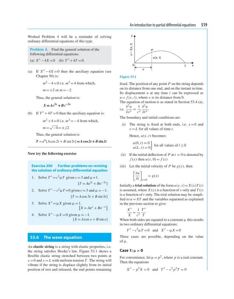
An elastic string is a string with elastic properties, i.e.
the string satisfies Hooke’s law. Figure 53.1 shows a
flexible elastic string stretched between two points at
x = 0 and x = L with uniform tension T . The string will
vibrate if the string is displace slightly from its initial
position of rest and released, the end points remaining
0
x
x
y
P
L
u(x, t )
u
5 f (x, t )
Figure 53.1
fixed. The position of any point P on the string depends
on its distance from one end, and on the instant in time.
Its displacement u at any time t can be expressed as
u = f (x, t ), where x is its distance from 0.
The equation of motion is as stated in Section 53.4 (a),
i.e.
∂ 2 u
∂x 2 =
1
c 2
∂ 2 u
∂t 2 .
The boundary and initial conditions are:
(i) The string is fixed at both ends, i.e. x = 0 and
x = L for all values of time t .
Hence, u(x, t ) becomes:
u(0, t ) = 0
u(L , t ) = 0
for all values of t ≥ 0
(ii) If the initial deflection of P at t = 0 is denoted by
f (x) then u(x, 0) = f (x)
(iii) Let the initial velocity of P be g(x), then
∂u
∂t
t =0
= g(x)
Initially a trial solution of the form u(x, t ) = X (x)T (t )
is assumed, where X (x) is a function of x only and T (t )
is a function of t only. The trial solution may be simplified to u = XT and the variables separated as explained
in the previous section to give:
X
X
=
1
c 2
T
T
When both sides are equated to a constant μ this results
in two ordinary differential equations:
T
− c
2
μT = 0 and X
− μX =0
Three cases are possible, depending on the value
of μ.
Case 1: μ > 0
For convenience, let μ = p 2 , where p is a real constant.
Then the equations
X
− p
2 X = 0 and T
− c
2 p
2 T = 0
Worked Problem 4 will be a reminder of solving
ordinary differential equations of this type.
Problem 4. Find the general solution of the
following differential equations:
(a) X − 4X =0 (b) T + 4T = 0.
(a) If X − 4X =0 then the auxiliary equation (see
Chapter 50) is:
m 2 − 4 = 0 i.e. m 2 = 4 from which,
m =+2 or m =−2
Thus, the general solution is:
X = Ae
2x
+ Be
−2x
(b) If T + 4T = 0 then the auxiliary equation is:
m 2 + 4 = 0 i.e. m 2 =−4 from which,
m =
√
−4 =± j 2
Thus, the general solution is:
T = e 0 {A cos 2t + B sin 2t } =A cos2t + B sin2t
Now try the following exercise
Exercise 200 Further problems on revising
the solution of ordinary differential equation
1. Solve T = c 2 μT given c = 3 and μ =1.
[T = Ae 3t + Be −3t ]
2. Solve T − c 2 μT =0 given c = 3 and μ =−1.
[T = A cos 3t + B sin 3t]
3. Solve X = μX given μ = 1.
X = Ae x + Be −x
4. Solve X − μX = 0 given μ =−1.
[X = A cos x + B sin x]
53.6 The wave equation
An elastic string is a string with elastic properties, i.e.
the string satisfies Hooke’s law. Figure 53.1 shows a
flexible elastic string stretched between two points at
x = 0 and x = L with uniform tension T . The string will
vibrate if the string is displace slightly from its initial
position of rest and released, the end points remaining
0
x
x
y
P
L
u(x, t )
u
5 f (x, t )
Figure 53.1
fixed. The position of any point P on the string depends
on its distance from one end, and on the instant in time.
Its displacement u at any time t can be expressed as
u = f (x, t ), where x is its distance from 0.
The equation of motion is as stated in Section 53.4 (a),
i.e.
∂ 2 u
∂x 2 =
1
c 2
∂ 2 u
∂t 2 .
The boundary and initial conditions are:
(i) The string is fixed at both ends, i.e. x = 0 and
x = L for all values of time t .
Hence, u(x, t ) becomes:
u(0, t ) = 0
u(L , t ) = 0
for all values of t ≥ 0
(ii) If the initial deflection of P at t = 0 is denoted by
f (x) then u(x, 0) = f (x)
(iii) Let the initial velocity of P be g(x), then
∂u
∂t
t =0
= g(x)
Initially a trial solution of the form u(x, t ) = X (x)T (t )
is assumed, where X (x) is a function of x only and T (t )
is a function of t only. The trial solution may be simplified to u = XT and the variables separated as explained
in the previous section to give:
X
X
=
1
c 2
T
T
When both sides are equated to a constant μ this results
in two ordinary differential equations:
T
− c
2
μT = 0 and X
− μX =0
Three cases are possible, depending on the value
of μ.
Case 1: μ > 0
For convenience, let μ = p 2 , where p is a real constant.
Then the equations
X
− p
2 X = 0 and T
− c
2 p
2 T = 0