

510 Higher Engineering Mathematics
i.e. y = AJ v (x)+ BJ −v (x)
= A
x
2
v
1
(v + 1)
−
x 2
2 2 (1!)(v + 2)
+
x 4
2 4 (2!)(v + 4)
− · · ·
+ B
x
2
−v
1
(1 −v)
−
x 2
2 2 (1!)(2 − v)
+
x 4
2 4 (2!)(3 −v)
− · · ·
In general terms: J v (x) =
x
2
v ∞
k=0
(−1) k x 2k
2 2k (k! ))(v+k+1)
and J −v (x) =
x
2
−v ∞
k=0
(−1) k x 2k
2 2k (k! ))(k − v + 1)
Another Bessel function
It may be shown that another series for J n (x) is given by:
J n (x) =
x
2
n
1
n!
−
1
(n + 1)!
x
2
2
+
1
(2! )(n + 2)!
x
2
4 − · · ·
From this series two commonly used function are
derived,
i.e. J 0 (x) =
1
(0! )
−
1
(1! ) 2
x
2
2 +
1
(2! ) 2
x
2
4
−
1
(3! ) 2
x
2
6 + · · ·
= 1 −
x 2
2 2 (1!)
2
+
x 4
2 4 (2!)
2
−
x 6
2 6 (3!)
2
+· · ·
and J 1 (x) =
x
2
1
(1! )
−
1
(1! )(2! )
x
2
2
+
1
(2! )(3! )
x
2
4 − · · ·
=
x
2
−
x 3
2 3 (1!)(2!)
+
x 5
2 5 (2!)(3!)
−
x
7
2 7 (3!)(4!)
+· · ·
Tables of Bessel functions are available for a range of
values of n and x, and in these, J 0 (x) and J 1 (x) are most
commonly used.
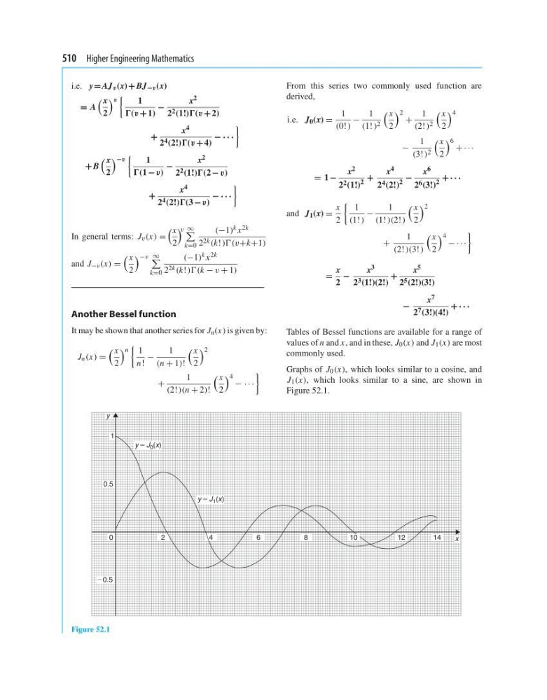
Graphs of J 0 (x), which looks similar to a cosine, and
J 1 (x), which looks similar to a sine, are shown in
Figure 52.1.
y ϭ J 0 (x)
y ϭ J 1 (x)
1
0.5
Ϫ0.5
0
2
4
6
8
12
14
x
y
10
Figure 52.1
i.e. y = AJ v (x)+ BJ −v (x)
= A
x
2
v
1
(v + 1)
−
x 2
2 2 (1!)(v + 2)
+
x 4
2 4 (2!)(v + 4)
− · · ·
+ B
x
2
−v
1
(1 −v)
−
x 2
2 2 (1!)(2 − v)
+
x 4
2 4 (2!)(3 −v)
− · · ·
In general terms: J v (x) =
x
2
v ∞
k=0
(−1) k x 2k
2 2k (k! ))(v+k+1)
and J −v (x) =
x
2
−v ∞
k=0
(−1) k x 2k
2 2k (k! ))(k − v + 1)
Another Bessel function
It may be shown that another series for J n (x) is given by:
J n (x) =
x
2
n
1
n!
−
1
(n + 1)!
x
2
2
+
1
(2! )(n + 2)!
x
2
4 − · · ·
From this series two commonly used function are
derived,
i.e. J 0 (x) =
1
(0! )
−
1
(1! ) 2
x
2
2 +
1
(2! ) 2
x
2
4
−
1
(3! ) 2
x
2
6 + · · ·
= 1 −
x 2
2 2 (1!)
2
+
x 4
2 4 (2!)
2
−
x 6
2 6 (3!)
2
+· · ·
and J 1 (x) =
x
2
1
(1! )
−
1
(1! )(2! )
x
2
2
+
1
(2! )(3! )
x
2
4 − · · ·
=
x
2
−
x 3
2 3 (1!)(2!)
+
x 5
2 5 (2!)(3!)
−
x
7
2 7 (3!)(4!)
+· · ·
Tables of Bessel functions are available for a range of
values of n and x, and in these, J 0 (x) and J 1 (x) are most
commonly used.
Graphs of J 0 (x), which looks similar to a cosine, and
J 1 (x), which looks similar to a sine, are shown in
Figure 52.1.
y ϭ J 0 (x)
y ϭ J 1 (x)
1
0.5
Ϫ0.5
0
2
4
6
8
12
14
x
y
10
Figure 52.1