

Chapter 38
Some applications of
integration
38.1 Introduction
There are a number of applications of integral calculus
in engineering. The determination of areas, mean and
r.m.s. values, volumes, centroids and second moments
of area and radius of gyration are included in this
chapter.
38.2 Areas under and between curves
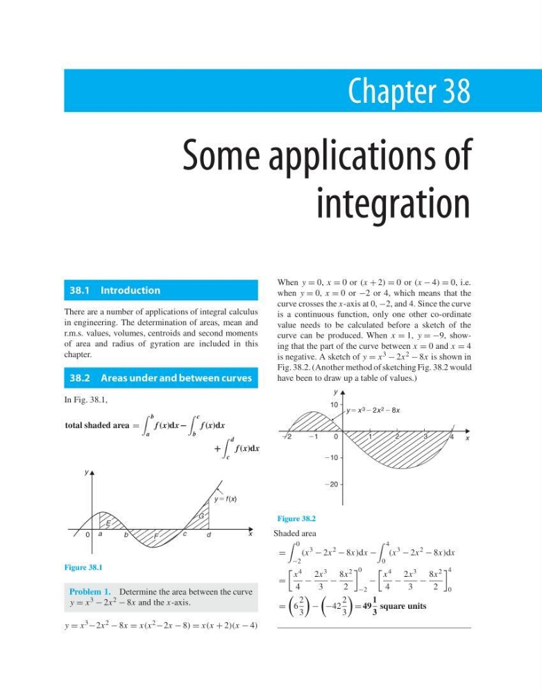
In Fig. 38.1,
total shaded area =
b
a
f (x)dx −
c
b
f (x)dx
+
d
c
f (x)dx
E
0
F
G
y
a
b
c
d
x
y 5 f (x)
Figure 38.1
Problem 1. Determine the area between the curve
y = x 3 − 2x 2 − 8x and the x-axis.
y = x 3 −2x 2 − 8x = x(x 2 −2x − 8) = x(x + 2)(x − 4)
When y = 0, x = 0 or (x + 2) = 0 or (x − 4) = 0, i.e.
when y = 0, x = 0 or −2 or 4, which means that the
curve crosses the x-axis at 0, −2, and 4. Since the curve
is a continuous function, only one other co-ordinate
value needs to be calculated before a sketch of the
curve can be produced. When x = 1, y = −9, showing that the part of the curve between x = 0 and x = 4
is negative. A sketch of y = x 3 − 2x 2 − 8x is shown in
Fig. 38.2. (Another method of sketching Fig. 38.2 would
have been to draw up a table of values.)
y
x
210
10
220
22
4
y 5 x 3 2 2x 2 2 8x
2
21
0
1
3
Figure 38.2
Shaded area
=
0
−2
(x
3
− 2x
2
− 8x)dx −
4
0
(x
3
− 2x
2
− 8x)dx
=
x 4
4
−
2x 3
3
−
8x 2
2
0
−2
−
x 4
4
−
2x 3
3
−
8x 2
2
4
0
=
6
2
3
−
−42
2
3
= 49
1
3
square units
Some applications of
integration
38.1 Introduction
There are a number of applications of integral calculus
in engineering. The determination of areas, mean and
r.m.s. values, volumes, centroids and second moments
of area and radius of gyration are included in this
chapter.
38.2 Areas under and between curves
In Fig. 38.1,
total shaded area =
b
a
f (x)dx −
c
b
f (x)dx
+
d
c
f (x)dx
E
0
F
G
y
a
b
c
d
x
y 5 f (x)
Figure 38.1
Problem 1. Determine the area between the curve
y = x 3 − 2x 2 − 8x and the x-axis.
y = x 3 −2x 2 − 8x = x(x 2 −2x − 8) = x(x + 2)(x − 4)
When y = 0, x = 0 or (x + 2) = 0 or (x − 4) = 0, i.e.
when y = 0, x = 0 or −2 or 4, which means that the
curve crosses the x-axis at 0, −2, and 4. Since the curve
is a continuous function, only one other co-ordinate
value needs to be calculated before a sketch of the
curve can be produced. When x = 1, y = −9, showing that the part of the curve between x = 0 and x = 4
is negative. A sketch of y = x 3 − 2x 2 − 8x is shown in
Fig. 38.2. (Another method of sketching Fig. 38.2 would
have been to draw up a table of values.)
y
x
210
10
220
22
4
y 5 x 3 2 2x 2 2 8x
2
21
0
1
3
Figure 38.2
Shaded area
=
0
−2
(x
3
− 2x
2
− 8x)dx −
4
0
(x
3
− 2x
2
− 8x)dx
=
x 4
4
−
2x 3
3
−
8x 2
2
0
−2
−
x 4
4
−
2x 3
3
−
8x 2
2
4
0
=
6
2
3
−
−42
2
3
= 49
1
3
square units