

336 Higher Engineering Mathematics
Thus
d y
dx
=
1
dx
d y
=
1
√
a 2 − x 2
i.e. when y = sin −1 x
a
then
dy
dx
=
1
√
a 2 − x 2
Since integration is the reverse process of differentiation then:
1
√
a 2 − x 2
dx = sin
−1 x
a
+ c
(iv) Given y = sin −1 f (x) the function of a function
rule may be used to find
dy
dx
Let u = f (x) then y = sin
−1 u
Then
du
dx
= f (x) and
dy
du
=
1
√
1 − u 2
(see para. (i))
Thus
dy
dx
=
dy
du
×
du
dx
=
1
√
1 − u 2
f
(x)
=
f (x)
1 −[ f (x)] 2
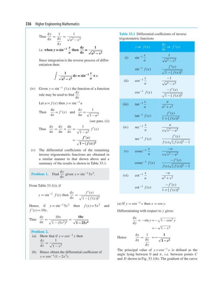
(v) The differential coefficients of the remaining
inverse trigonometric functions are obtained in
a similar manner to that shown above and a
summary of the results is shown in Table 33.1.
Problem 1. Find
dy
dx
given y = sin −1 5x 2 .
From Table 33.1(i), if
y = sin
−1 f (x) then
dy
dx
=
f (x)
1 − [ f (x)] 2
Hence, if y = sin −1 5x 2 then f (x) = 5x 2 and
f (x) = 10x.
Thus
dy
dx
=
10x
1 − (5x 2 ) 2
=
10x
√
1 −25x 4
Problem 2.
(a) Show that if y = cos −1 x then
dy
dx
=
1
√
1 − x 2
(b) Hence obtain the differential coefficient of
y = cos −1 (1 − 2x 2 ).
Table 33.1 Differential coefficients of inverse
trigonometric functions
y or f (x)
dy
dx
or f (x)
(i)
sin −1 x
a
1
√
a 2 − x 2
sin −1 f (x)
f (x)
1 − [ f (x)] 2
(ii)
cos −1 x
a
−1
√
a 2 − x 2
cos
−1 f (x)
− f (x)
1 − [ f (x)] 2
(iii)
tan −1 x
a
a
a 2 + x 2
tan −1 f (x)
f (x)
1 + [ f (x)] 2
(iv)
sec −1 x
a
a
x
√
x 2 − a 2
sec −1 f (x)
f
(x)
f (x)
[ f (x)] 2 − 1
(v)
cosec −1 x
a
−a
x
√
x 2 − a 2
cosec
−1 f (x)
− f (x)
f (x)
[ f (x)] 2 − 1
(vi)
cot −1 x
a
−a
a 2 + x 2
cot −1 f (x)
− f (x)
1 + [ f (x)] 2
(a) If y = cos −1 x then x = cos y.
Differentiating with respect to y gives:
dx
dy
= −sin y =−
1 − cos 2 y
=−
√
1 − x 2
Hence
dy
dx
=
1
dx
dy
= −
1
√
1 −x 2
The principal value of y = cos −1 x is defined as the
angle lying between 0 and π, i.e. between points C
and D shown in Fig. 33.1(b). The gradient of the curve
Thus
d y
dx
=
1
dx
d y
=
1
√
a 2 − x 2
i.e. when y = sin −1 x
a
then
dy
dx
=
1
√
a 2 − x 2
Since integration is the reverse process of differentiation then:
1
√
a 2 − x 2
dx = sin
−1 x
a
+ c
(iv) Given y = sin −1 f (x) the function of a function
rule may be used to find
dy
dx
Let u = f (x) then y = sin
−1 u
Then
du
dx
= f (x) and
dy
du
=
1
√
1 − u 2
(see para. (i))
Thus
dy
dx
=
dy
du
×
du
dx
=
1
√
1 − u 2
f
(x)
=
f (x)
1 −[ f (x)] 2
(v) The differential coefficients of the remaining
inverse trigonometric functions are obtained in
a similar manner to that shown above and a
summary of the results is shown in Table 33.1.
Problem 1. Find
dy
dx
given y = sin −1 5x 2 .
From Table 33.1(i), if
y = sin
−1 f (x) then
dy
dx
=
f (x)
1 − [ f (x)] 2
Hence, if y = sin −1 5x 2 then f (x) = 5x 2 and
f (x) = 10x.
Thus
dy
dx
=
10x
1 − (5x 2 ) 2
=
10x
√
1 −25x 4
Problem 2.
(a) Show that if y = cos −1 x then
dy
dx
=
1
√
1 − x 2
(b) Hence obtain the differential coefficient of
y = cos −1 (1 − 2x 2 ).
Table 33.1 Differential coefficients of inverse
trigonometric functions
y or f (x)
dy
dx
or f (x)
(i)
sin −1 x
a
1
√
a 2 − x 2
sin −1 f (x)
f (x)
1 − [ f (x)] 2
(ii)
cos −1 x
a
−1
√
a 2 − x 2
cos
−1 f (x)
− f (x)
1 − [ f (x)] 2
(iii)
tan −1 x
a
a
a 2 + x 2
tan −1 f (x)
f (x)
1 + [ f (x)] 2
(iv)
sec −1 x
a
a
x
√
x 2 − a 2
sec −1 f (x)
f
(x)
f (x)
[ f (x)] 2 − 1
(v)
cosec −1 x
a
−a
x
√
x 2 − a 2
cosec
−1 f (x)
− f (x)
f (x)
[ f (x)] 2 − 1
(vi)
cot −1 x
a
−a
a 2 + x 2
cot −1 f (x)
− f (x)
1 + [ f (x)] 2
(a) If y = cos −1 x then x = cos y.
Differentiating with respect to y gives:
dx
dy
= −sin y =−
1 − cos 2 y
=−
√
1 − x 2
Hence
dy
dx
=
1
dx
dy
= −
1
√
1 −x 2
The principal value of y = cos −1 x is defined as the
angle lying between 0 and π, i.e. between points C
and D shown in Fig. 33.1(b). The gradient of the curve