

Chapter 18
Functions and their curves
18.1 Standard curves
When a mathematical equation is known, co-ordinates
may be calculated for a limited range of values, and
the equation may be represented pictorially as a graph,
within this range of calculated values. Sometimes it
is useful to show all the characteristic features of an
equation, and in this case a sketch depicting the equation can be drawn, in which all the important features
are shown, but the accurate plotting of points is less
important. This technique is called ‘curve sketching’
and can involve the use of differential calculus, with,
for example, calculations involving turning points.
If, say, y depends on, say, x, then y is said to be a function of x and the relationship is expressed as y = f (x); x
is called the independent variable and y is the dependent
variable.
In engineering and science, corresponding values are
obtained as a result of tests or experiments.
Here is a brief resumé of standard curves, some of
which have been met earlier in this text.
(i) Straight Line
The general equation of a straight line is y = mx + c,
where m is the gradient
i.e.
d y
dx
and c is the y-axis
intercept.
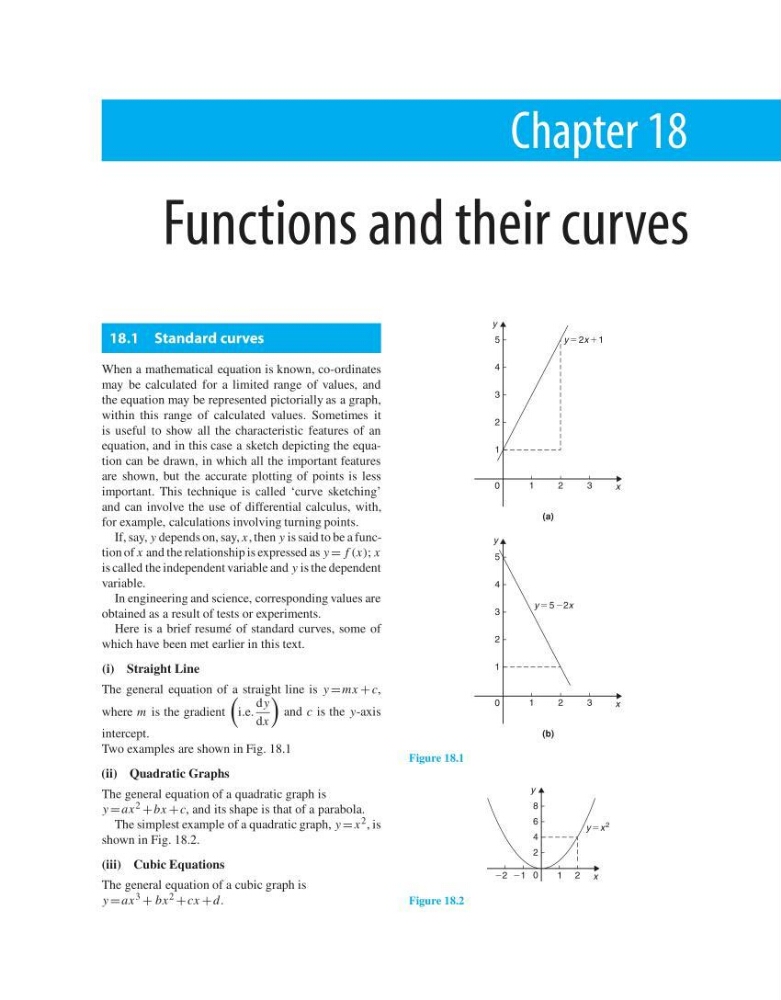
Two examples are shown in Fig. 18.1
(ii) Quadratic Graphs
The general equation of a quadratic graph is
y = ax 2 + bx + c, and its shape is that of a parabola.
The simplest example of a quadratic graph, y = x 2 , is
shown in Fig. 18.2.
(iii) Cubic Equations
The general equation of a cubic graph is
y = ax 3 + bx 2 + cx + d.
5
4
3
2
1
3
2
1
0
y 5 2x 1 1
y
x
5
(a)
(b)
4
3
2
1
3
2
1
0
y 5 5 22x
y
x
Figure 18.1
8
6
4
2
22 21
1
0
2 x
y
y 5x
2
Figure 18.2
Functions and their curves
18.1 Standard curves
When a mathematical equation is known, co-ordinates
may be calculated for a limited range of values, and
the equation may be represented pictorially as a graph,
within this range of calculated values. Sometimes it
is useful to show all the characteristic features of an
equation, and in this case a sketch depicting the equation can be drawn, in which all the important features
are shown, but the accurate plotting of points is less
important. This technique is called ‘curve sketching’
and can involve the use of differential calculus, with,
for example, calculations involving turning points.
If, say, y depends on, say, x, then y is said to be a function of x and the relationship is expressed as y = f (x); x
is called the independent variable and y is the dependent
variable.
In engineering and science, corresponding values are
obtained as a result of tests or experiments.
Here is a brief resumé of standard curves, some of
which have been met earlier in this text.
(i) Straight Line
The general equation of a straight line is y = mx + c,
where m is the gradient
i.e.
d y
dx
and c is the y-axis
intercept.
Two examples are shown in Fig. 18.1
(ii) Quadratic Graphs
The general equation of a quadratic graph is
y = ax 2 + bx + c, and its shape is that of a parabola.
The simplest example of a quadratic graph, y = x 2 , is
shown in Fig. 18.2.
(iii) Cubic Equations
The general equation of a cubic graph is
y = ax 3 + bx 2 + cx + d.
5
4
3
2
1
3
2
1
0
y 5 2x 1 1
y
x
5
(a)
(b)
4
3
2
1
3
2
1
0
y 5 5 22x
y
x
Figure 18.1
8
6
4
2
22 21
1
0
2 x
y
y 5x
2
Figure 18.2