Section 9.3 Finite-State Machines
747
table 9.12
d 1
d 2
s 0
0
0
s 1
0
1
s 2
1
0
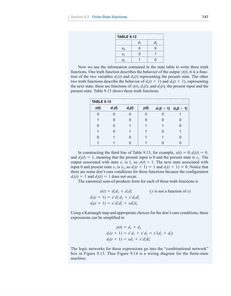
Now we use the information contained in the state table to write three truth
functions. One truth function describes the behavior of the output y(t); it is a function of the two variables d 1 (t) and d 2 (t) representing the present state. The other
two truth functions describe the behavior of d 1 (t + 1) and d 2 (t + 1), representing
the next state; these are functions of x(t), d 1 (t), and d 2 (t), the present input and the
present state. Table 9.13 shows these truth functions.
table 9.13
x(t)
d 1 (t)
d 2 (t)
y(t)
d 1 (t + 1) d 2 (t + 1)
0
0
0
0
0
1
1
0
0
0
0
0
0
0
1
1
1
0
1
0
1
1
0
1
0
1
0
1
1
0
1
1
0
1
0
0
In constructing the third line of Table 9.13, for example, x(t) = 0, d 1 (t) = 0,
and d 2 (t) = 1, meaning that the present input is 0 and the present state is s 1 . The
output associated with state s 1 is 1, so y(t) = 1. The next state associated with
input 0 and present state s 1 is s 2 , so d 1 (t + 1) = 1 and d 2 (t + 1) = 0. Notice that
there are some don’t-care conditions for these functions because the configuration
d 1 (t) = 1 and d 2 (t) = 1 does not occur.
The canonical sum-of-products form for each of these truth functions is
y(t) = d 1 ′d 2 + d 1 d 2 ′
( y is not a function of x)
d 1 (t + 1) = x′d 1 ′ d 2 + x′ d 1 d 2 ′
d 2 (t + 1) = x′d 1 ′d 2 ′ + xd 1 ′d 2
Using a Karnaugh map and appropriate choices for the don’t-care conditions, these
expressions can be simplified to
y(t) = d 1 + d 2
d 1 (t + 1) = x′d 1 + x′d 2 = x′(d 1 + d 2 )
d 2 (t + 1) = xd 2 + x′d 1 ′d 2 ′
The logic networks for these expressions go into the “combinational network”
box in Figure 9.13. Thus Figure 9.14 is a wiring diagram for the finite-state
machine.