

454
Relations, Functions, and Matrices
E
c 11 c 12 …
c 1n
d 1
0
c 22 …
c 2n
d 1
(
0
0
… c (n−1)(n−1) c (n−1)n d n−1
0
0
…
0
c nn
d n
U
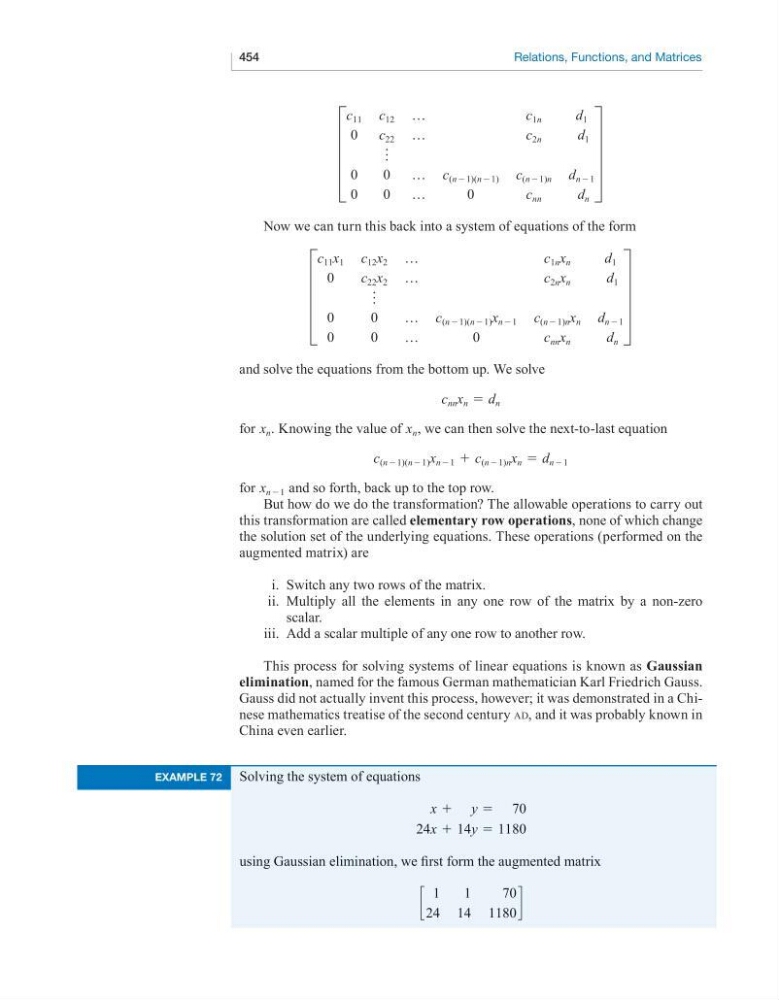
Now we can turn this back into a system of equations of the form
E
c 11 x 1 c 12 x 2 …
c 1n x n
d 1
0
c 22 x 2 …
c 2n x n
d 1
(
0
0
… c (n−1)(n−1) x n−1 c (n−1)n x n d n−1
0
0
…
0
c nn x n
d n
U
and solve the equations from the bottom up. We solve
c nn x n = d n
for x n . Knowing the value of x n , we can then solve the next-to-last equation
c (n−1)(n−1) x n−1 + c (n−1)n x n = d n−1
for x n−1 and so forth, back up to the top row.
But how do we do the transformation? The allowable operations to carry out
this transformation are called elementary row operations, none of which change
the solution set of the underlying equations. These operations (performed on the
augmented matrix) are
i. Switch any two rows of the matrix.
ii. Multiply all the elements in any one row of the matrix by a non-zero
scalar.
iii. Add a scalar multiple of any one row to another row.
This process for solving systems of linear equations is known as Gaussian
elimination, named for the famous German mathematician Karl Friedrich Gauss.
Gauss did not actually invent this process, however; it was demonstrated in a Chinese mathematics treatise of the second century ad, and it was probably known in
China even earlier.
example 72
Solving the system of equations
x + y = 70
24x + 14y = 1180
using Gaussian elimination, we first form the augmented matrix
c
1
1
70
24 14 1180
d
Relations, Functions, and Matrices
E
c 11 c 12 …
c 1n
d 1
0
c 22 …
c 2n
d 1
(
0
0
… c (n−1)(n−1) c (n−1)n d n−1
0
0
…
0
c nn
d n
U
Now we can turn this back into a system of equations of the form
E
c 11 x 1 c 12 x 2 …
c 1n x n
d 1
0
c 22 x 2 …
c 2n x n
d 1
(
0
0
… c (n−1)(n−1) x n−1 c (n−1)n x n d n−1
0
0
…
0
c nn x n
d n
U
and solve the equations from the bottom up. We solve
c nn x n = d n
for x n . Knowing the value of x n , we can then solve the next-to-last equation
c (n−1)(n−1) x n−1 + c (n−1)n x n = d n−1
for x n−1 and so forth, back up to the top row.
But how do we do the transformation? The allowable operations to carry out
this transformation are called elementary row operations, none of which change
the solution set of the underlying equations. These operations (performed on the
augmented matrix) are
i. Switch any two rows of the matrix.
ii. Multiply all the elements in any one row of the matrix by a non-zero
scalar.
iii. Add a scalar multiple of any one row to another row.
This process for solving systems of linear equations is known as Gaussian
elimination, named for the famous German mathematician Karl Friedrich Gauss.
Gauss did not actually invent this process, however; it was demonstrated in a Chinese mathematics treatise of the second century ad, and it was probably known in
China even earlier.
example 72
Solving the system of equations
x + y = 70
24x + 14y = 1180
using Gaussian elimination, we first form the augmented matrix
c
1
1
70
24 14 1180
d