

Section 4.6 Probability
313
Binomial distributions
Consider an event that has only two possible outcomes, success or failure. The
probability of success is p and the probability of failure q = 1 − p. Our wellknown coin toss would fit this description because there are only two possible
outcomes. Such an event is called a Bernoulli trial or Bernoulli experiment
after the eighteenth-century Swiss mathematician Jacob (or James) Bernoulli.
However, a single Bernoulli trial is not of much interest; instead we want to talk
about a finite series of Bernoulli trials, each of which has the same probability p of
success (hence the same probability q = 1 − p of failure). Because the probability
of success does not vary, the various trials are mutually independent events.
Without specifically describing the sample space S, we can define a random
variable X as the number of successful outcomes that occur in the n trials. X can
range from 0 (no successful outcomes) to n (all successful outcomes). We can determine the probability of k successful outcomes out of n trials as follows:
Assume the k successes (and (n − k) failures) occur in some specific pattern.
For example if k = 3 and n = 4, one pattern would look like S-F-S-S. The probability of a success is p, the probability of a failure is q. Because the n trials are
mutually independent, we can multiply their probabilities, giving p
k
q
n−k
. But this
is only one pattern of k successes; how many patterns are there? Exactly the number of ways we can select k out of n items, C(n, k). So the probability of k successful outcomes out of n trials is
P(k) = C(n, k)p
k
q
n−k
We have therefore determined a probability distribution for the various values of
X, as shown in this table:
X = k
0
1
2
c
k
c
n
P(k)
C(n, 0) p
0
q
n C(n,1)pq
n−1
C(n,2)p
2
q
n−2
C(n,k)p
k
q
n−k
C(n,n)p
n
q
0
Look at the values in this probability distribution. They are the terms in the expansion of (q + p)
n
. Hence this is called a binomial distribution.
Notice that because q + p = 1, the sum of the probability distribution terms
equals 1
n
= 1. This makes sense because the various values of X are all disjoint so
the probability of their union is the sum of their individual probabilities. But the
union covers all possible outcomes, so its probability is 1.
example 75
A fair coin is tossed three times, with heads being considered a success, tails being
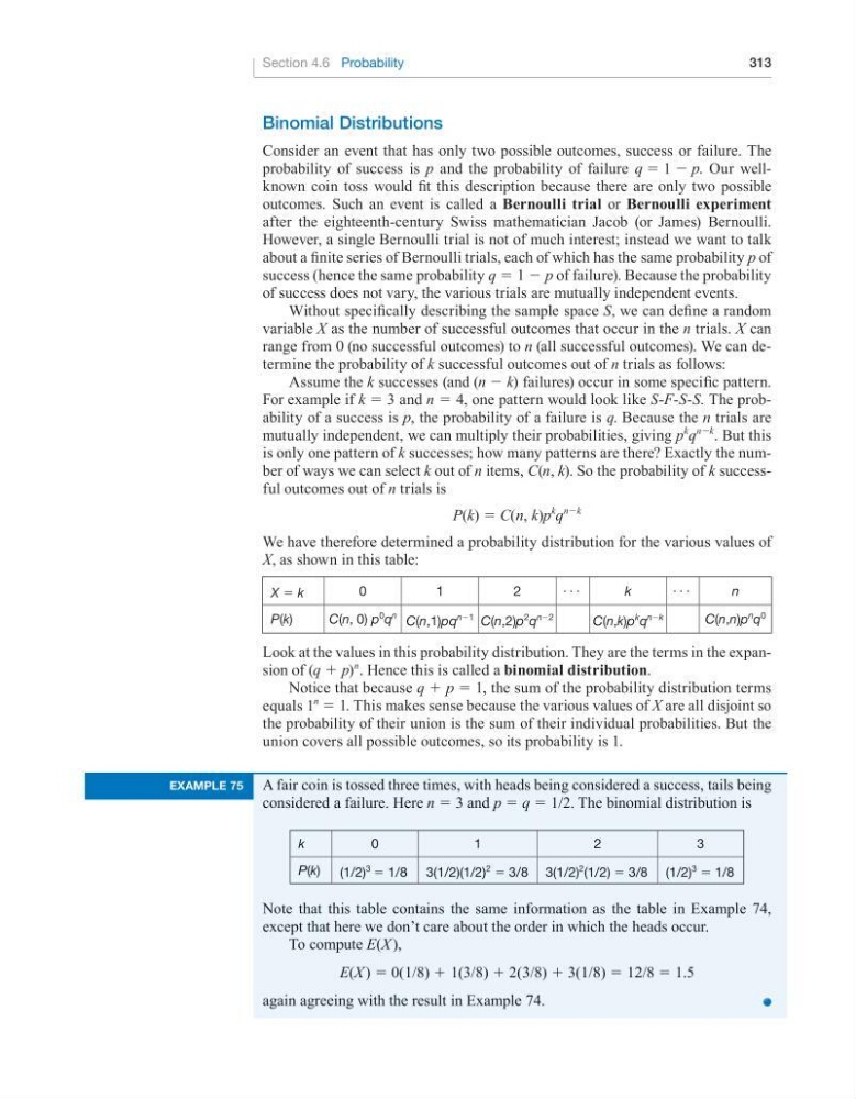
considered a failure. Here n = 3 and p = q = 1/2. The binomial distribution is
k
0
1
2
3
P(k) (1/2)
3
= 1/8 3(1/2)(1/2)
2
= 3/8 3(1/2)
2 (1/2) = 3/8 (1/2)
3
= 1/8
Note that this table contains the same information as the table in Example 74,
except that here we don’t care about the order in which the heads occur.
To compute E(X ),
E(X ) = 0(1/8) + 1(3/8) + 2(3/8) + 3(1/8) = 12/8 = 1.5
again agreeing with the result in Example 74.
313
Binomial distributions
Consider an event that has only two possible outcomes, success or failure. The
probability of success is p and the probability of failure q = 1 − p. Our wellknown coin toss would fit this description because there are only two possible
outcomes. Such an event is called a Bernoulli trial or Bernoulli experiment
after the eighteenth-century Swiss mathematician Jacob (or James) Bernoulli.
However, a single Bernoulli trial is not of much interest; instead we want to talk
about a finite series of Bernoulli trials, each of which has the same probability p of
success (hence the same probability q = 1 − p of failure). Because the probability
of success does not vary, the various trials are mutually independent events.
Without specifically describing the sample space S, we can define a random
variable X as the number of successful outcomes that occur in the n trials. X can
range from 0 (no successful outcomes) to n (all successful outcomes). We can determine the probability of k successful outcomes out of n trials as follows:
Assume the k successes (and (n − k) failures) occur in some specific pattern.
For example if k = 3 and n = 4, one pattern would look like S-F-S-S. The probability of a success is p, the probability of a failure is q. Because the n trials are
mutually independent, we can multiply their probabilities, giving p
k
q
n−k
. But this
is only one pattern of k successes; how many patterns are there? Exactly the number of ways we can select k out of n items, C(n, k). So the probability of k successful outcomes out of n trials is
P(k) = C(n, k)p
k
q
n−k
We have therefore determined a probability distribution for the various values of
X, as shown in this table:
X = k
0
1
2
c
k
c
n
P(k)
C(n, 0) p
0
q
n C(n,1)pq
n−1
C(n,2)p
2
q
n−2
C(n,k)p
k
q
n−k
C(n,n)p
n
q
0
Look at the values in this probability distribution. They are the terms in the expansion of (q + p)
n
. Hence this is called a binomial distribution.
Notice that because q + p = 1, the sum of the probability distribution terms
equals 1
n
= 1. This makes sense because the various values of X are all disjoint so
the probability of their union is the sum of their individual probabilities. But the
union covers all possible outcomes, so its probability is 1.
example 75
A fair coin is tossed three times, with heads being considered a success, tails being
considered a failure. Here n = 3 and p = q = 1/2. The binomial distribution is
k
0
1
2
3
P(k) (1/2)
3
= 1/8 3(1/2)(1/2)
2
= 3/8 3(1/2)
2 (1/2) = 3/8 (1/2)
3
= 1/8
Note that this table contains the same information as the table in Example 74,
except that here we don’t care about the order in which the heads occur.
To compute E(X ),
E(X ) = 0(1/8) + 1(3/8) + 2(3/8) + 3(1/8) = 12/8 = 1.5
again agreeing with the result in Example 74.