

Time Domain Representation of Continuous and Discrete Signals
81
figure(2)
% reconstructions
f25 = 0;
for k = 1:1:26;
fr25 = fd(k)*sinc(Fs*(t-k*Ts));
f25 = f25+fr25;
end
subplot(3,1,1)
plot(t,f25,’ko-’,t,fa,’ks-.’); legend(‘sinc-reconst’,’f(t)’);
title(‘Reconstruction of f(t) ‘)
ylabel(‘Amplitude’)
subplot(3,1,2)
stem(nTs,fd);hold on;
stairs(nTs,fd); ylabel(‘Amplitude’);legend(‘stairs’)
subplot(3,1,3)
y = spline(nTs,fd,t);
plot(nTs(1:2.5:26.5),y); legend(‘spline’);
ylabel(‘Amplitude’)
xlabel(‘time (sec)’)
figure(3)
error=abs(fa-f25);
plot(t,error);ylabel(‘magnitude’)
title(‘error(t) = abs [f(t) - Reconstruction (Sums(sinc))]’)
xlabel(‘time(sec)’)
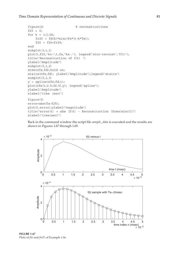
Back in the command window the script fi le sample_data is executed and the results are
shown in Figures 1.67 through 1.69.
FIGURE 1.67
Plots of f(t) and f(nT) of Example 1.16.
0
0.5
1
1.5
2
2.5
3
3.5
4
4.5
5
× 10 −3
× 10 −4
× 10
−4
time index n (msec)
0
0.5
1
1.5
2
2.5
3
3.5
4
4.5
5
× 10
−3
time t (msec)
4
2
0
Amplitude
4
2
0
Amplitude
f(t) versus t
f(t) sample with Ts=.2msec.
CRC_47760_CH001.indd 81
CRC_47760_CH001.indd 81
7/25/2008 4:16:26 PM
7/25/2008 4:16:26 PM
81
figure(2)
% reconstructions
f25 = 0;
for k = 1:1:26;
fr25 = fd(k)*sinc(Fs*(t-k*Ts));
f25 = f25+fr25;
end
subplot(3,1,1)
plot(t,f25,’ko-’,t,fa,’ks-.’); legend(‘sinc-reconst’,’f(t)’);
title(‘Reconstruction of f(t) ‘)
ylabel(‘Amplitude’)
subplot(3,1,2)
stem(nTs,fd);hold on;
stairs(nTs,fd); ylabel(‘Amplitude’);legend(‘stairs’)
subplot(3,1,3)
y = spline(nTs,fd,t);
plot(nTs(1:2.5:26.5),y); legend(‘spline’);
ylabel(‘Amplitude’)
xlabel(‘time (sec)’)
figure(3)
error=abs(fa-f25);
plot(t,error);ylabel(‘magnitude’)
title(‘error(t) = abs [f(t) - Reconstruction (Sums(sinc))]’)
xlabel(‘time(sec)’)
Back in the command window the script fi le sample_data is executed and the results are
shown in Figures 1.67 through 1.69.
FIGURE 1.67
Plots of f(t) and f(nT) of Example 1.16.
0
0.5
1
1.5
2
2.5
3
3.5
4
4.5
5
× 10 −3
× 10 −4
× 10
−4
time index n (msec)
0
0.5
1
1.5
2
2.5
3
3.5
4
4.5
5
× 10
−3
time t (msec)
4
2
0
Amplitude
4
2
0
Amplitude
f(t) versus t
f(t) sample with Ts=.2msec.
CRC_47760_CH001.indd 81
CRC_47760_CH001.indd 81
7/25/2008 4:16:26 PM
7/25/2008 4:16:26 PM