

80
Practical MATLAB
® Applications for Engineers
Example 1.16
Let f(t) = te
−1000t u(t)
Create the script fi le sample_data that returns the following plots:
a. f(t) versus t, over the range 0 ≤ t ≤ 5 ms
b. f(nT) versus nt, for T = 0.2 ms, over the range 1 ≤ n ≤ 26
c. Reconstruct f(t) from f(nT) using
i. Summations of sinc functions (emulating a low-pass fi lter)
ii. Stair function
iii. Spine function
d. error(t) versus t, for the reconstruction process when a low-pass fi lter is used, where
error t
f t
fn nT
c F t nT
F
T
s
s
S
n
N
S
S
( )
( )
(
)sin [ (
)] ,
ϭ
Ϫ
Ϫ
ϭ
ϭ
ϭ
1
26
1
∑
for
MATLAB Solution
% Script file: sample _ data
t = 0:0.0005:0.005;
% 26 time samples
fa = t.*exp(-1000.*t);
figure(1)
subplot(2,1,1)
plot(t,fa);title(‘f(t) vs t’)
ylabel(‘Amplitude’);xlabel(‘time t (msec)’);
subplot(2,1,2)
Ts = 0.0002; n = 0:1:25; Fs=1/Ts;
nTs = n*Ts;
fd = nTs.*exp(-1000*nTs);
stem(nTs,fd);hold on;
plot(nTs,fd);
title(‘f(t) sample with Ts=.2msec.’);
ylabel(‘Amplitude’); xlabel(‘time index n (msec)’)
20
18
16
14
12
10
time index n
8
6
4
2
0
−1
−0.5
0
1
2
1.5
0.5
error
error=[mov.ave/2terms] versus t
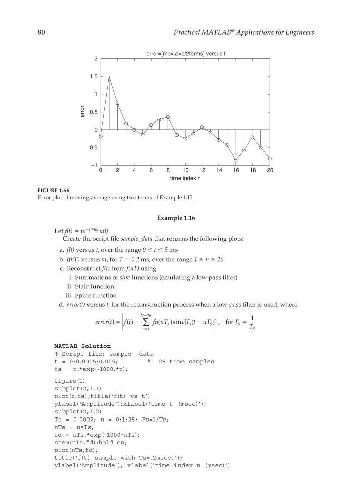
FIGURE 1.66
Error plot of moving average using two terms of Example 1.15.
CRC_47760_CH001.indd 80
CRC_47760_CH001.indd 80
7/25/2008 4:16:26 PM
7/25/2008 4:16:26 PM
Practical MATLAB
® Applications for Engineers
Example 1.16
Let f(t) = te
−1000t u(t)
Create the script fi le sample_data that returns the following plots:
a. f(t) versus t, over the range 0 ≤ t ≤ 5 ms
b. f(nT) versus nt, for T = 0.2 ms, over the range 1 ≤ n ≤ 26
c. Reconstruct f(t) from f(nT) using
i. Summations of sinc functions (emulating a low-pass fi lter)
ii. Stair function
iii. Spine function
d. error(t) versus t, for the reconstruction process when a low-pass fi lter is used, where
error t
f t
fn nT
c F t nT
F
T
s
s
S
n
N
S
S
( )
( )
(
)sin [ (
)] ,
ϭ
Ϫ
Ϫ
ϭ
ϭ
ϭ
1
26
1
∑
for
MATLAB Solution
% Script file: sample _ data
t = 0:0.0005:0.005;
% 26 time samples
fa = t.*exp(-1000.*t);
figure(1)
subplot(2,1,1)
plot(t,fa);title(‘f(t) vs t’)
ylabel(‘Amplitude’);xlabel(‘time t (msec)’);
subplot(2,1,2)
Ts = 0.0002; n = 0:1:25; Fs=1/Ts;
nTs = n*Ts;
fd = nTs.*exp(-1000*nTs);
stem(nTs,fd);hold on;
plot(nTs,fd);
title(‘f(t) sample with Ts=.2msec.’);
ylabel(‘Amplitude’); xlabel(‘time index n (msec)’)
20
18
16
14
12
10
time index n
8
6
4
2
0
−1
−0.5
0
1
2
1.5
0.5
error
error=[mov.ave/2terms] versus t
FIGURE 1.66
Error plot of moving average using two terms of Example 1.15.
CRC_47760_CH001.indd 80
CRC_47760_CH001.indd 80
7/25/2008 4:16:26 PM
7/25/2008 4:16:26 PM