

Time Domain Representation of Continuous and Discrete Signals
67
axis([-1 5 -.2 4.3]);
subplot(2,2,3);
f3=-1.*fn;
% creates -f(n)
plot(n,f3);title(‘-f(n) vs. n’);
axis([-1 5 -2.3 .2]);
ylabel(‘Amplitude’);xlabel(‘time index n’);
subplot(2,2,4)
shiftn = n+2;plot(shiftn, fn)
title(‘f(n-2) vs. n’);
ylabel(‘Amplitude’);xlabel(‘time index n’);
axis([0 5 -.5 2.5]);
disp(‘*********** RESULTS ARE : ************************’)
Energy _ fn = sum(fnsquare)
disp(‘
’)
Power _ fn = Energyfn/length(n)
% asuming, f (n) is periodic T=20
disp(‘(in joules and watts)’)
disp(‘*************************************************’)
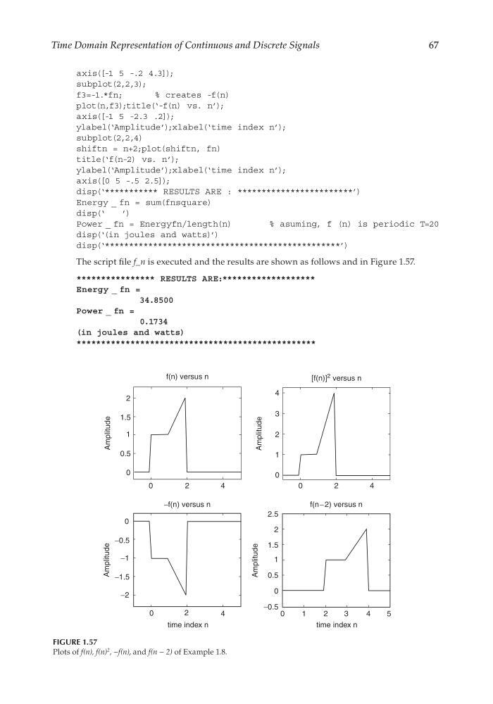
The script fi le f_n is executed and the results are shown as follows and in Figure 1.57.
**************** RESULTS ARE:*******************
Energy _ fn =
34.8500
Power _ fn =
0.1734
(in joules and watts)
*************************************************
f(n) versus n
−f(n) versus n
f(n− 2) versus n
[f(n)] 2 versus n
2
1.5
0.5
0
0
−0.5
2.5
1.5
0.5
0
0
−0.5
1
2
−1
−1.5
−2
0
2
4
0
2
4
1
Amplitude
Amplitude
Amplitude
Amplitude
4
3
2
1
0
0
2
4
time index n
1
2
3
4
5
time index n
FIGURE 1.57
Plots of f(n), f(n)
2
, −f(n), and f(n − 2) of Example 1.8.
CRC_47760_CH001.indd 67
CRC_47760_CH001.indd 67
7/25/2008 4:16:24 PM
7/25/2008 4:16:24 PM
67
axis([-1 5 -.2 4.3]);
subplot(2,2,3);
f3=-1.*fn;
% creates -f(n)
plot(n,f3);title(‘-f(n) vs. n’);
axis([-1 5 -2.3 .2]);
ylabel(‘Amplitude’);xlabel(‘time index n’);
subplot(2,2,4)
shiftn = n+2;plot(shiftn, fn)
title(‘f(n-2) vs. n’);
ylabel(‘Amplitude’);xlabel(‘time index n’);
axis([0 5 -.5 2.5]);
disp(‘*********** RESULTS ARE : ************************’)
Energy _ fn = sum(fnsquare)
disp(‘
’)
Power _ fn = Energyfn/length(n)
% asuming, f (n) is periodic T=20
disp(‘(in joules and watts)’)
disp(‘*************************************************’)
The script fi le f_n is executed and the results are shown as follows and in Figure 1.57.
**************** RESULTS ARE:*******************
Energy _ fn =
34.8500
Power _ fn =
0.1734
(in joules and watts)
*************************************************
f(n) versus n
−f(n) versus n
f(n− 2) versus n
[f(n)] 2 versus n
2
1.5
0.5
0
0
−0.5
2.5
1.5
0.5
0
0
−0.5
1
2
−1
−1.5
−2
0
2
4
0
2
4
1
Amplitude
Amplitude
Amplitude
Amplitude
4
3
2
1
0
0
2
4
time index n
1
2
3
4
5
time index n
FIGURE 1.57
Plots of f(n), f(n)
2
, −f(n), and f(n − 2) of Example 1.8.
CRC_47760_CH001.indd 67
CRC_47760_CH001.indd 67
7/25/2008 4:16:24 PM
7/25/2008 4:16:24 PM