

Time Domain Representation of Continuous and Discrete Signals
61
MATLAB Solution
% Script file: graphs
t = -5:.01:5; t0 = 0;
u = stepfun(t,t0);
f1 = 4.5*exp(-1.4.*t).*cos(8.3.*t+1.25).*u;
subplot(2,1,1);
plot(t,f1);axis([-5 5 -4 5]);
title(‘[f1(t)= 4.5 exp(-1.4.*t).*cos(8.3 *t + 1.25).*u(t)] vs. t’);
ylabel(‘Amplitude [f1(t)]’); xlabel(‘t (time)’);
f2 = fliplr(f1);
subplot(2,1,2);
plot(t,f2);axis([-5 5 -4 5]);
title(‘[f2(t)= f1(-t)] vs. t’);
ylabel(‘Amplitude [f2(t)]’); xlabel(‘t (time)’);
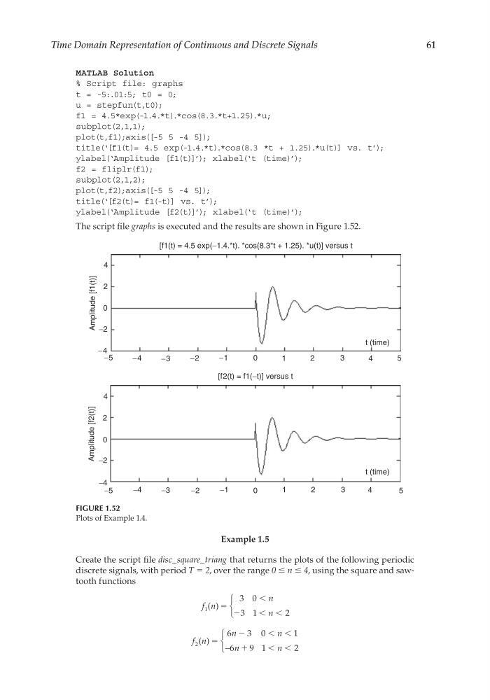
The script fi le graphs is executed and the results are shown in Figure 1.52.
Example 1.5
Create the script fi le disc_square_triang that returns the plots of the following periodic
discrete signals, with period T = 2, over the range 0 ≤ n ≤ 4, using the square and sawtooth functions
f n
n
n
1
3 0
3 1
2
( ) ϭ
Ͻ
Ϫ
Ͻ Ͻ
f n
n
n
n
n
2
6
3 0
1
6
9 1
2
( ) ϭ
ϩ
Ϫ
Ͻ Ͻ
Ͻ Ͻ
−
[f1(t) = 4.5 exp(−1.4.*t). *cos(8.3*t + 1.25). *u(t)] versus t
4
2
0
−2
−4
−5
−4
−3
−2
−1
0
1
2
3
4
5
t (time)
t (time)
Amplitude [f1(t)]
Amplitude [f2(t)]
[f2(t) = f1(−t)] versus t
4
2
0
−2
−4
−5
−4
−3
−2
−1
0
1
2
3
4
5
FIGURE 1.52
Plots of Example 1.4.
CRC_47760_CH001.indd 61
CRC_47760_CH001.indd 61
7/25/2008 4:16:23 PM
7/25/2008 4:16:23 PM
61
MATLAB Solution
% Script file: graphs
t = -5:.01:5; t0 = 0;
u = stepfun(t,t0);
f1 = 4.5*exp(-1.4.*t).*cos(8.3.*t+1.25).*u;
subplot(2,1,1);
plot(t,f1);axis([-5 5 -4 5]);
title(‘[f1(t)= 4.5 exp(-1.4.*t).*cos(8.3 *t + 1.25).*u(t)] vs. t’);
ylabel(‘Amplitude [f1(t)]’); xlabel(‘t (time)’);
f2 = fliplr(f1);
subplot(2,1,2);
plot(t,f2);axis([-5 5 -4 5]);
title(‘[f2(t)= f1(-t)] vs. t’);
ylabel(‘Amplitude [f2(t)]’); xlabel(‘t (time)’);
The script fi le graphs is executed and the results are shown in Figure 1.52.
Example 1.5
Create the script fi le disc_square_triang that returns the plots of the following periodic
discrete signals, with period T = 2, over the range 0 ≤ n ≤ 4, using the square and sawtooth functions
f n
n
n
1
3 0
3 1
2
( ) ϭ
Ͻ
Ϫ
Ͻ Ͻ
f n
n
n
n
n
2
6
3 0
1
6
9 1
2
( ) ϭ
ϩ
Ϫ
Ͻ Ͻ
Ͻ Ͻ
−
[f1(t) = 4.5 exp(−1.4.*t). *cos(8.3*t + 1.25). *u(t)] versus t
4
2
0
−2
−4
−5
−4
−3
−2
−1
0
1
2
3
4
5
t (time)
t (time)
Amplitude [f1(t)]
Amplitude [f2(t)]
[f2(t) = f1(−t)] versus t
4
2
0
−2
−4
−5
−4
−3
−2
−1
0
1
2
3
4
5
FIGURE 1.52
Plots of Example 1.4.
CRC_47760_CH001.indd 61
CRC_47760_CH001.indd 61
7/25/2008 4:16:23 PM
7/25/2008 4:16:23 PM