

60
Practical MATLAB
® Applications for Engineers
urev = fliplr(un);n1 = -5;
un _ 5 = stepfun(n, n1); fn1=3*(urev .* un _ 5);
subplot(2,1,1)
stem(n,fn1);hold on; plot(n,yzero)
title(‘f1(n) vs. n’);
ylabel(‘Amplitude [f1(n)]’); xlabel(‘Discrete time n’)
un1=stepfun(n,1); fn2=3*(un _ 5 -un1);
axis([-10 10 -1 4])
subplot(2,1,2)
stem(n, fn2);hold on; plot(n,yzero);
title(‘f2(n) vs. n’);
ylabel(‘Amplitude [f1(n)]’); xlabel(‘ Discrete time n ‘);
axis([-10 10 -1 4])
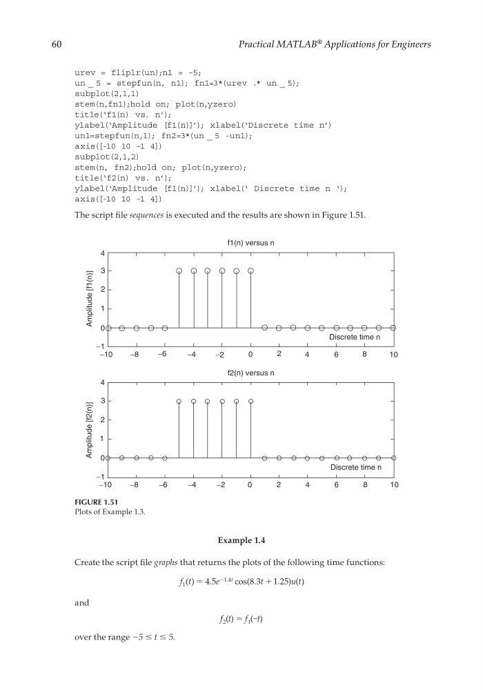
The script fi le sequences is executed and the results are shown in Figure 1.51.
Example 1.4
Create the script fi le graphs that returns the plots of the following time functions:
f t
e
t
u t
t
1
1 4
4 5
8 3 1 25
( )
.
cos( .
. ) ( )
.
ϭ
ϩ
Ϫ
and
f 2 (t) = f 1 (–t)
over the range −5 ≤ t ≤ 5.
FIGURE 1.51
Plots of Example 1.3.
f1(n) versus n
f2(n) versus n
4
3
2
1
−1
−10
−8
−6
−4
−2
0
2
4
6
Discrete time n
8
10
0
Amplitude [f1(n)]
Amplitude [f2(n)]
4
3
2
1
0
−1
−10
−8
−6
−4
−2
0
2
4
6
8
1 0
Discrete time n
CRC_47760_CH001.indd 60
CRC_47760_CH001.indd 60
7/25/2008 4:16:23 PM
7/25/2008 4:16:23 PM
Practical MATLAB
® Applications for Engineers
urev = fliplr(un);n1 = -5;
un _ 5 = stepfun(n, n1); fn1=3*(urev .* un _ 5);
subplot(2,1,1)
stem(n,fn1);hold on; plot(n,yzero)
title(‘f1(n) vs. n’);
ylabel(‘Amplitude [f1(n)]’); xlabel(‘Discrete time n’)
un1=stepfun(n,1); fn2=3*(un _ 5 -un1);
axis([-10 10 -1 4])
subplot(2,1,2)
stem(n, fn2);hold on; plot(n,yzero);
title(‘f2(n) vs. n’);
ylabel(‘Amplitude [f1(n)]’); xlabel(‘ Discrete time n ‘);
axis([-10 10 -1 4])
The script fi le sequences is executed and the results are shown in Figure 1.51.
Example 1.4
Create the script fi le graphs that returns the plots of the following time functions:
f t
e
t
u t
t
1
1 4
4 5
8 3 1 25
( )
.
cos( .
. ) ( )
.
ϭ
ϩ
Ϫ
and
f 2 (t) = f 1 (–t)
over the range −5 ≤ t ≤ 5.
FIGURE 1.51
Plots of Example 1.3.
f1(n) versus n
f2(n) versus n
4
3
2
1
−1
−10
−8
−6
−4
−2
0
2
4
6
Discrete time n
8
10
0
Amplitude [f1(n)]
Amplitude [f2(n)]
4
3
2
1
0
−1
−10
−8
−6
−4
−2
0
2
4
6
8
1 0
Discrete time n
CRC_47760_CH001.indd 60
CRC_47760_CH001.indd 60
7/25/2008 4:16:23 PM
7/25/2008 4:16:23 PM