

Analog and Digital Filters
609
Example 6.3
Given the second-order fi lter shown in Figure 6.37.
a. Determine by hand the transfer function H(s) = V o (s)/V i (s).
b. Verify using MATLAB that the circuit of Figure 6.37 corresponds to a normalized
LPF by obtaining the magnitude and phase plots of H(w).
c. Make the following substitutions corresponding to the frequency shifting property: R = R N , L = L N /2, and C = C N /2 and obtain its transfer function H(s), its magnitude and phase plots, and its numerator and denominator polynomial coeffi cients.
d. Using the transformations of part (c), obtain magnitude and phase plots of the
nonnormalized fi lter H(w) corresponding to an LPF and verify that the fi lter’s
cutoff frequency is w c = 2 rad/s.
e. Use the MATLAB function lp2lp on the fi lter transfer function of part (b) to shift the
cutoff frequency to w c = 2 rad/s. Obtain the system transfer function H(s), its magnitude and phase plots, and its numerator and denominator polynomial coeffi cients.
f. Implement the fi lter specs of part (b) using a Butterworth, second-order normalized LPF. Obtain its transfer function H(s), its magnitude and phase plots, and its
numerator and denominator polynomial coeffi cients.
g. Using the MATLAB function lp2lp transform the normalized LPF of part (f) into a
denormalized LPF with cutoff frequency of w c = 2 rad/s. Obtain its transfer function H(s), its magnitude and phase plots, and its numerator and denominator polynomial coeffi cients.
h. Implement the normalized Butterworth LPF of part (f) using electrical elements.
i. Implement the denormilized Butterworth LPF of part (g) using electrical elements
(RLC).
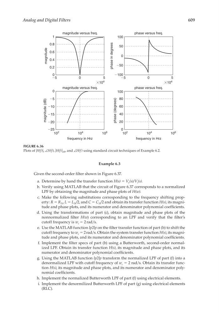
FIGURE 6.36
Plots of ͉H(f)͉, ∠H(f), ͉H(f)͉ dB , and ∠H(f) using standard circuit techniques of Example 6.2.
0
magnitude versus freq.
magnitude versus freq.
phase versus freq.
phase versus freq.
frequency in Hrz
frequency in Hrz
0
0.2
magnitude
magnitude (dB)
0.4
0.6
0.8
1
5
Ϫ5
5
Ϫ5
Ϫ15
Ϫ20
Ϫ25
Ϫ10
Ϫ5
0
phase (degrees)
phase in degrees
80
60
40
20
0
100
Ϫ100
Ϫ50
0
50
100
0
10
4
10
2
ϫ10
4
ϫ10
4
10
6
10
4
10
2
10
6
CRC_47760_CH006.indd 609
CRC_47760_CH006.indd 609
7/23/2008 2:26:45 PM
7/23/2008 2:26:45 PM