

574
Practical MATLAB
® Applications for Engineers
"
"
H (jw)
a
ϭ
ϩ
1
1
2 1 2
w
w p
n
/
Table 6.3 provides the transfer function H(jw) for the case of LP normalized fi lters
of the order n = 1, 2, 3, 4, and 5.
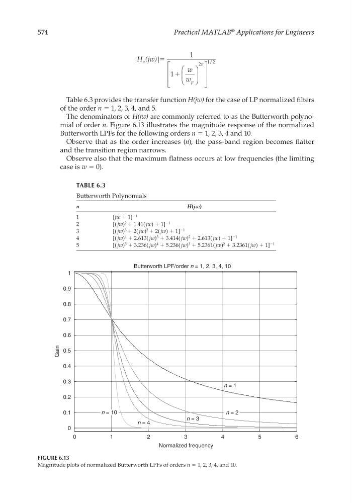
The denominators of H(jw) are commonly referred to as the Butterworth polynomial of order n. Figure 6.13 illustrates the magnitude response of the normalized
Butterworth LPFs for the following orders n = 1, 2, 3, 4 and 10.
Observe that as the order increases (n), the pass-band region becomes fl atter
and the transition region narrows.
Observe also that the maximum fl atness occurs at low frequencies (the limiting
case is w = 0).
TABLE 6.3
Butterworth Polynomials
n
H (jw)
1
[ jw + 1]
−1
2
[( jw)
2 + 1.41( jw) + 1]
−1
3
[( jw)
3 + 2( jw)
2 + 2( jw) + 1]
−1
4
[( jw)
4 + 2.613( jw)
3 + 3.414( jw)
2 + 2.613( jw) + 1]
−1
5
[( jw)
5 + 3.236( jw)
4 + 5.236( jw)
3 + 5.2361( jw)
2 + 3.2361( jw) + 1]
−1
FIGURE 6.13
Magnitude plots of normalized Butterworth LPFs of orders n = 1, 2, 3, 4, and 10.
0
1
2
3
4
5
6
0
0.1
0.2
0.3
0.4
0.5
0.6
0.7
0.8
0.9
1
Normalized frequency
Gain
Butterworth LPF/order n = 1, 2, 3, 4, 10
n = 3
n = 1
n = 10
n = 4
n = 2
CRC_47760_CH006.indd 574
CRC_47760_CH006.indd 574
7/23/2008 2:26:33 PM
7/23/2008 2:26:33 PM