

512
Practical MATLAB
® Applications for Engineers
−4
−3
−2
−1
0
1
2
3
4
1.6
1.4
1.2
1
0.8
0.6
−4
−3
−2
−1
0
frequency W
1
2
3
4
0.4
Amplitude
Amplitude
0.2
0
−0.2
−0.6
real [DTFT[f1(n)] versus W
imag [DTFT[f1(n)] versus W
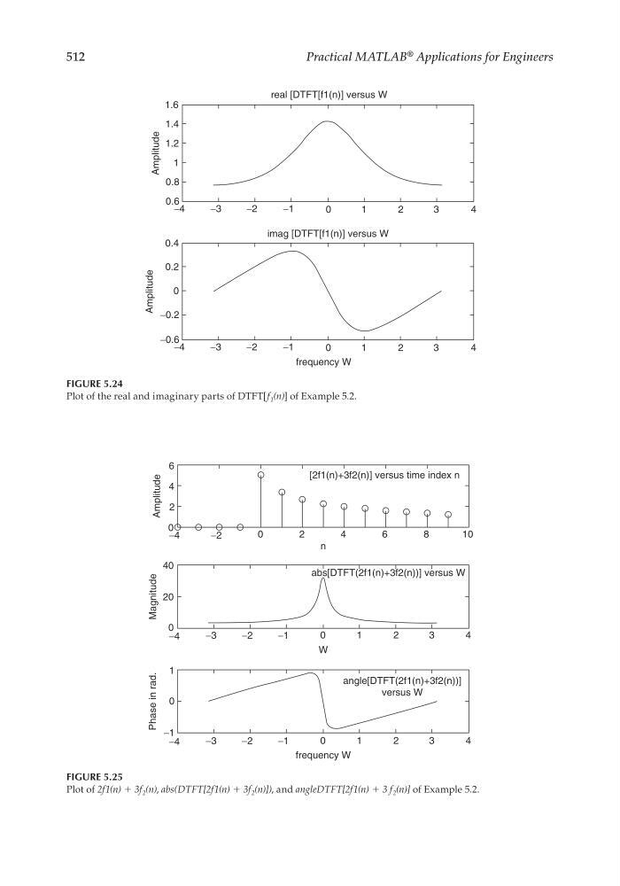
FIGURE 5.24
Plot of the real and imaginary parts of DTFT[f 1 (n)] of Example 5.2.
−4
−2
0
0
2
40
20
0
0
Phase in rad.
1
−1
Amplitude
Magnitude
4
6
2
4
6
8
1 0
−4
−3
−2
−1
0
2
1
3
4
−4
−3
−2
−1
0
2
1
3
4
frequency W
angle[DTFT(2f1(n)+3f2(n))]
versus W
abs[DTFT(2f1(n)+3f2(n))] versus W
[2f1(n)+3f2(n)] versus time index n
n
W
FIGURE 5.25
Plot of 2f1(n) + 3f 2 (n), abs(DTFT[2f1(n) + 3f 2 (n)]), and angleDTFT[2f1(n) + 3 f 2 (n)] of Example 5.2.
CRC_47760_CH005.indd 512
CRC_47760_CH005.indd 512
7/23/2008 1:47:31 PM
7/23/2008 1:47:31 PM
Practical MATLAB
® Applications for Engineers
−4
−3
−2
−1
0
1
2
3
4
1.6
1.4
1.2
1
0.8
0.6
−4
−3
−2
−1
0
frequency W
1
2
3
4
0.4
Amplitude
Amplitude
0.2
0
−0.2
−0.6
real [DTFT[f1(n)] versus W
imag [DTFT[f1(n)] versus W
FIGURE 5.24
Plot of the real and imaginary parts of DTFT[f 1 (n)] of Example 5.2.
−4
−2
0
0
2
40
20
0
0
Phase in rad.
1
−1
Amplitude
Magnitude
4
6
2
4
6
8
1 0
−4
−3
−2
−1
0
2
1
3
4
−4
−3
−2
−1
0
2
1
3
4
frequency W
angle[DTFT(2f1(n)+3f2(n))]
versus W
abs[DTFT(2f1(n)+3f2(n))] versus W
[2f1(n)+3f2(n)] versus time index n
n
W
FIGURE 5.25
Plot of 2f1(n) + 3f 2 (n), abs(DTFT[2f1(n) + 3f 2 (n)]), and angleDTFT[2f1(n) + 3 f 2 (n)] of Example 5.2.
CRC_47760_CH005.indd 512
CRC_47760_CH005.indd 512
7/23/2008 1:47:31 PM
7/23/2008 1:47:31 PM