

DTFT, DFT, ZT, and FFT
483
c. For the causal signal f(n), if f(n) = 0 for n < 0, then the exterior of the circle
defi ned by the pole with the largest magnitude constitutes the ROC.
d. For the noncausal signal f(n), if f(n) ≠ 0 for n < 0, the ROC is inside the circle
defi ned by the pole with the smallest magnitude.
R.5.69 The ROC of a stable, LTI system includes the unit circle since that fact would
imply that the impulse response is absolutely summable.
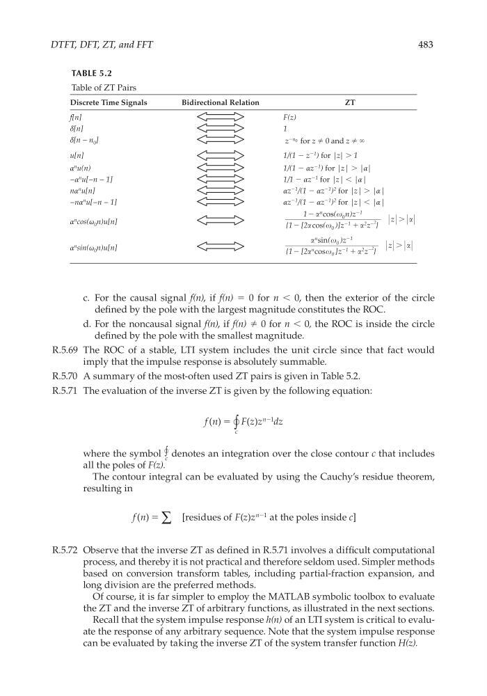
R.5.70 A summary of the most-often used ZT pairs is given in Table 5.2.
R.5.71 The evaluation of the inverse ZT is given by the following equation:
f n
F z z dz
n
c
( )
( )
ϭ
Ϫ1
∫
where the symbol c
∫ denotes an integration over the close contour c that includes
all the poles of F(z).
The contour integral can be evaluated by using the Cauchy’s residue theorem,
resulting in
f n
F z z
c
n
( )
[
( )
]
ϭ
Ϫ
residues of
at the poles inside
∑
1
R.5.72 Observe that the inverse ZT as defi ned in R.5.71 involves a diffi cult computational
process, and thereby it is not practical and therefore seldom used. Simpler methods
based on conversion transform tables, including partial-fraction expansion, and
long division are the preferred methods.
Of course, it is far simpler to employ the MATLAB symbolic toolbox to evaluate
the ZT and the inverse ZT of arbitrary functions, as illustrated in the next sections.
Recall that the system impulse response h(n) of an LTI system is critical to evaluate the response of any arbitrary sequence. Note that the system impulse response
can be evaluated by taking the inverse ZT of the system transfer function H(z).
TABLE 5.2
Table of ZT Pairs
Discrete Time Signals
Bidirectional Relation
ZT
f[n]
F(z)
δ[n]
1
δ[n − n 0 ]
z
z
z
n
Ϫ
ϱ
0 for
0 and
u[n]
1/(1 − z
−1
) for |z| > 1
α
n u(n)
1/(1 − αz
−1 ) for |z| > |α|
−α
n
u[−n − 1]
1/1 − αz
−1 for |z| < |α|
nα
n
u[n]
αz
−1
/(1 − αz
−1
)
2 for |z| > |α|
−nα
n u[−n − 1]
αz
−1
/(1 − αz
−1
)
2 for |z| < |α|
α
n cos(ω 0 n)u[n]
1
(
)
{1 [2
( )]
}
1
1
2
2
Ϫ
Ϫ
ϩ
Ϫ
Ϫ
Ϫ
n
n z
z
z
z
cos
cos
0
0
Ͼ
α
n sin(ω 0 n)u[n]
n
n
z
z
z
z
sin
cos
( )
{1 [2
]
}
0
1
0
1
2
2
Ϫ
Ϫ
Ϫ
Ϫ
ϩ
Ͼ
CRC_47760_CH005.indd 483
CRC_47760_CH005.indd 483
7/23/2008 1:47:23 PM
7/23/2008 1:47:23 PM
483
c. For the causal signal f(n), if f(n) = 0 for n < 0, then the exterior of the circle
defi ned by the pole with the largest magnitude constitutes the ROC.
d. For the noncausal signal f(n), if f(n) ≠ 0 for n < 0, the ROC is inside the circle
defi ned by the pole with the smallest magnitude.
R.5.69 The ROC of a stable, LTI system includes the unit circle since that fact would
imply that the impulse response is absolutely summable.
R.5.70 A summary of the most-often used ZT pairs is given in Table 5.2.
R.5.71 The evaluation of the inverse ZT is given by the following equation:
f n
F z z dz
n
c
( )
( )
ϭ
Ϫ1
∫
where the symbol c
∫ denotes an integration over the close contour c that includes
all the poles of F(z).
The contour integral can be evaluated by using the Cauchy’s residue theorem,
resulting in
f n
F z z
c
n
( )
[
( )
]
ϭ
Ϫ
residues of
at the poles inside
∑
1
R.5.72 Observe that the inverse ZT as defi ned in R.5.71 involves a diffi cult computational
process, and thereby it is not practical and therefore seldom used. Simpler methods
based on conversion transform tables, including partial-fraction expansion, and
long division are the preferred methods.
Of course, it is far simpler to employ the MATLAB symbolic toolbox to evaluate
the ZT and the inverse ZT of arbitrary functions, as illustrated in the next sections.
Recall that the system impulse response h(n) of an LTI system is critical to evaluate the response of any arbitrary sequence. Note that the system impulse response
can be evaluated by taking the inverse ZT of the system transfer function H(z).
TABLE 5.2
Table of ZT Pairs
Discrete Time Signals
Bidirectional Relation
ZT
f[n]
F(z)
δ[n]
1
δ[n − n 0 ]
z
z
z
n
Ϫ
ϱ
0 for
0 and
u[n]
1/(1 − z
−1
) for |z| > 1
α
n u(n)
1/(1 − αz
−1 ) for |z| > |α|
−α
n
u[−n − 1]
1/1 − αz
−1 for |z| < |α|
nα
n
u[n]
αz
−1
/(1 − αz
−1
)
2 for |z| > |α|
−nα
n u[−n − 1]
αz
−1
/(1 − αz
−1
)
2 for |z| < |α|
α
n cos(ω 0 n)u[n]
1
(
)
{1 [2
( )]
}
1
1
2
2
Ϫ
Ϫ
ϩ
Ϫ
Ϫ
Ϫ
n
n z
z
z
z
cos
cos
0
0
Ͼ
α
n sin(ω 0 n)u[n]
n
n
z
z
z
z
sin
cos
( )
{1 [2
]
}
0
1
0
1
2
2
Ϫ
Ϫ
Ϫ
Ϫ
ϩ
Ͼ
CRC_47760_CH005.indd 483
CRC_47760_CH005.indd 483
7/23/2008 1:47:23 PM
7/23/2008 1:47:23 PM