

474
Practical MATLAB
® Applications for Engineers
R.5.48 The power of ZT is that any difference equation can be easily transformed into
an algebraic expression, which can then be easily solved by algebraic manipulations. This transformation can be accomplished based on two important properties, which can be easily learned and applied. They are
a. Linearity
b. Time shift
It is obvious that ZT is linear, since DTFT is also linear. Then, based on the linearity principles
Z a f n
a f n
Z a f n
Z a f n
a F z
a F z
[
( )
( )]
[
( )]
[
( )]
( )
( )
1 1
2 2
1 1
2 2
1 1
2 2
ϩ
ϭ
ϩ
ϭ
ϩ
and the time-shift property yields
Z f n n
z F z
n
n
[ (
)]
( )
Ϫ
ϭ
Ϫ
0
for any integer
0
0
R.5. 49 Let us consider the case where the input to a discrete system is f(n) = r(n) = r
n (a ramp),
and its system impulse response is h(n). Then the output g(n) can be evaluated by
g(n) = f(n) ⊗ h(n) (convolution of f(n) with h(n) in time), analyzed as follows:
g n
r h n k
k
k
( )
(
)
ϭ
Ϫ
ϭϪϱ
ϩϱ
∑
or
g n
r h k
n k
k
( )
( )
ϭ
Ϫ
ϭϪϱ
ϩϱ
∑
and
g n
r
h k r
n
k
k
( )
( )
ϭ
Ϫ
ϭϪϱ
ϩϱ
∑
where clearly
r h k
H z
k
kϭϱ
ϩϱ
ϭ
∑ ( ) ( )
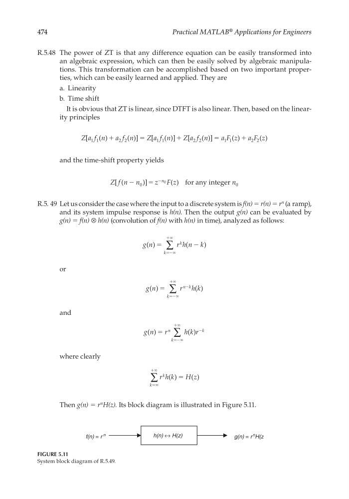
Then g(n) = r
n H(z). Its block diagram is illustrated in Figure 5.11.
FIGURE 5.11
System block diagram of R.5.49.
f(n) = r n
g(n) = r
n H(z
h(n) ↔ H(z)
CRC_47760_CH005.indd 474
CRC_47760_CH005.indd 474
7/23/2008 1:47:20 PM
7/23/2008 1:47:20 PM
Practical MATLAB
® Applications for Engineers
R.5.48 The power of ZT is that any difference equation can be easily transformed into
an algebraic expression, which can then be easily solved by algebraic manipulations. This transformation can be accomplished based on two important properties, which can be easily learned and applied. They are
a. Linearity
b. Time shift
It is obvious that ZT is linear, since DTFT is also linear. Then, based on the linearity principles
Z a f n
a f n
Z a f n
Z a f n
a F z
a F z
[
( )
( )]
[
( )]
[
( )]
( )
( )
1 1
2 2
1 1
2 2
1 1
2 2
ϩ
ϭ
ϩ
ϭ
ϩ
and the time-shift property yields
Z f n n
z F z
n
n
[ (
)]
( )
Ϫ
ϭ
Ϫ
0
for any integer
0
0
R.5. 49 Let us consider the case where the input to a discrete system is f(n) = r(n) = r
n (a ramp),
and its system impulse response is h(n). Then the output g(n) can be evaluated by
g(n) = f(n) ⊗ h(n) (convolution of f(n) with h(n) in time), analyzed as follows:
g n
r h n k
k
k
( )
(
)
ϭ
Ϫ
ϭϪϱ
ϩϱ
∑
or
g n
r h k
n k
k
( )
( )
ϭ
Ϫ
ϭϪϱ
ϩϱ
∑
and
g n
r
h k r
n
k
k
( )
( )
ϭ
Ϫ
ϭϪϱ
ϩϱ
∑
where clearly
r h k
H z
k
kϭϱ
ϩϱ
ϭ
∑ ( ) ( )
Then g(n) = r
n H(z). Its block diagram is illustrated in Figure 5.11.
FIGURE 5.11
System block diagram of R.5.49.
f(n) = r n
g(n) = r
n H(z
h(n) ↔ H(z)
CRC_47760_CH005.indd 474
CRC_47760_CH005.indd 474
7/23/2008 1:47:20 PM
7/23/2008 1:47:20 PM