

448
Practical MATLAB
® Applications for Engineers
t
t
t
t
−2
0
1
2
−1
−1
+1
1
f 7 (t )
f 4 (t )
f 6 (t )
f 5 (t )
f 3 (t )
f 2 (t )
f 1 (t )
2
0
1
1
0
2
−2
0
2
t
t
t
1
−1
−1
0
3
3
0
2
3
3
2
1
1.5
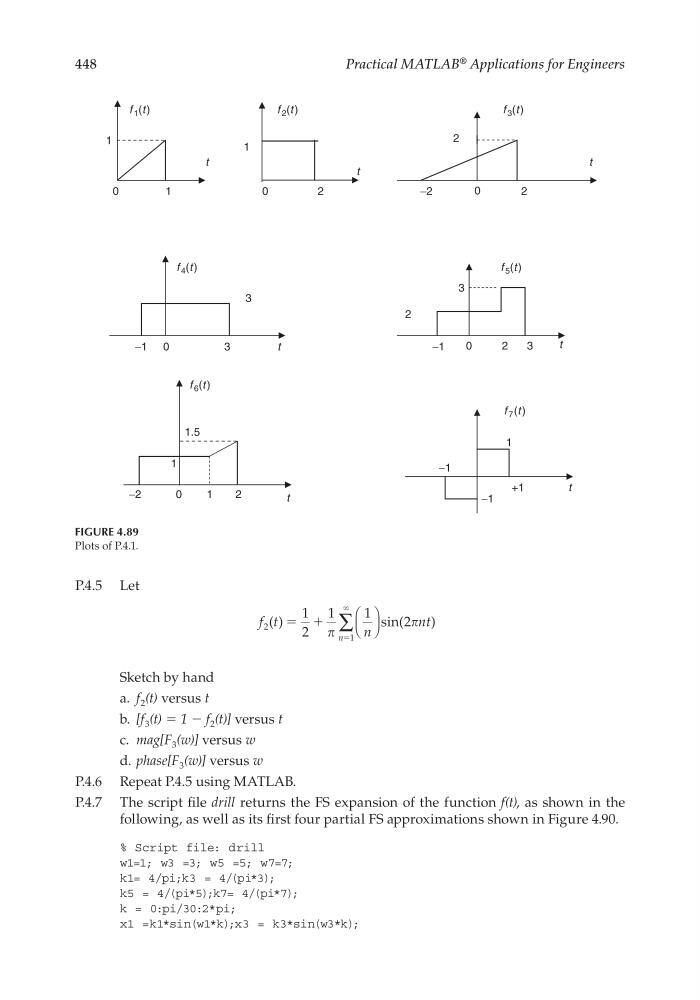
FIGURE 4.89
Plots of P.4.1.
P.4.5 Let
f t
n
nt
n
2
1
1
2
1
1
2
( )
sin(
)
ϭ ϩ
∑
ϭ
ϱ
Sketch by hand
a. f 2 (t) versus t
b. [f 3 (t) = 1 − f 2 (t)] versus t
c. mag[F 3 (w)] versus w
d. phase[F 3 (w)] versus w
P.4.6 Repeat P.4.5 using MATLAB.
P.4.7 The script fi le drill returns the FS expansion of the function f(t), as shown in the
following, as well as its fi rst four partial FS approximations shown in Figure 4.90.
% Script file: drill
w1=1; w3 =3; w5 =5; w7=7;
k1= 4/pi;k3 = 4/(pi*3);
k5 = 4/(pi*5);k7= 4/(pi*7);
k = 0:pi/30:2*pi;
x1 =k1*sin(w1*k);x3 = k3*sin(w3*k);
CRC_47760_CH004.indd 448
CRC_47760_CH004.indd 448
7/28/2008 12:26:24 PM
7/28/2008 12:26:24 PM
Practical MATLAB
® Applications for Engineers
t
t
t
t
−2
0
1
2
−1
−1
+1
1
f 7 (t )
f 4 (t )
f 6 (t )
f 5 (t )
f 3 (t )
f 2 (t )
f 1 (t )
2
0
1
1
0
2
−2
0
2
t
t
t
1
−1
−1
0
3
3
0
2
3
3
2
1
1.5
FIGURE 4.89
Plots of P.4.1.
P.4.5 Let
f t
n
nt
n
2
1
1
2
1
1
2
( )
sin(
)
ϭ ϩ
∑
ϭ
ϱ
Sketch by hand
a. f 2 (t) versus t
b. [f 3 (t) = 1 − f 2 (t)] versus t
c. mag[F 3 (w)] versus w
d. phase[F 3 (w)] versus w
P.4.6 Repeat P.4.5 using MATLAB.
P.4.7 The script fi le drill returns the FS expansion of the function f(t), as shown in the
following, as well as its fi rst four partial FS approximations shown in Figure 4.90.
% Script file: drill
w1=1; w3 =3; w5 =5; w7=7;
k1= 4/pi;k3 = 4/(pi*3);
k5 = 4/(pi*5);k7= 4/(pi*7);
k = 0:pi/30:2*pi;
x1 =k1*sin(w1*k);x3 = k3*sin(w3*k);
CRC_47760_CH004.indd 448
CRC_47760_CH004.indd 448
7/28/2008 12:26:24 PM
7/28/2008 12:26:24 PM