

Fourier and Laplace
433
V 1 (s) = 50/s
V 2 (s) =
ZL1(s) = s
ZC1(s) = 2/s
R1(s) = 2
R 2 (s) = 3
R3 (s) = 4
ZL 2(s) = 3 s
ZC 2(s) = 3/s
I 1 (s)
I 2 (s)
2 V
9 V
3/s
4/s
15
s 2 +9
−
−
+
+
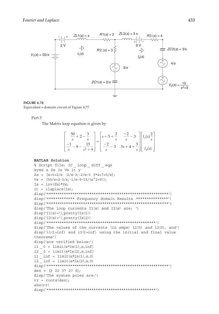
FIGURE 4.78
Equivalent s-domain circuit of Figure 4.77.
Part 3
The Matrix loop equation is given by
50 2
3
1 9
15
9
5
2
2 3
2 3 3
4
5
2
s
s
s
s
s
s
s
s
s
s
ϩ
ϩ
ϭ
ϩ ϩ
ϩ ϩ
Ϫ
Ϫ Ϫ Ϫ
Ϫ Ϫ
Ϫ Ϫ
I s
s
I s
1
2
2
( )
( )
MATLAB Solution
% Script file: IC _ loop _ diff _ eqs
syms s Zs Is Vs it y
Zs = [s+5+2/s -2/s-3;-2/s-3 3*s+7+5/s];
Vs = [50/s+2-3/s;-1/s-9-15/(s^2+9)];
Is = inv(Zs)*Vs;
it = ilaplace(Is);
disp(‘*********************************************************’)
disp(‘************* Frequency domain Results ***************’)
disp(‘*********************************************************’)
disp(‘The loop currents I1(s) and I2(s) are: ‘)
disp(‘I1(s)=’),pretty(Is(1))
disp(‘I2(s)=’),pretty(Is(2))
disp(‘***************************************************’)
disp(‘The values of the currents (in amps) i1(0) and i2(0), and’)
disp(‘i1(t=inf) and i2(t=inf) using the initial and final value
theorems’)
disp(‘are verified below:’)
i1 _ 0 = limit(s*Is(1),s,inf)
i2 _ 0 = limit(s*Is(2),s,inf)
i1 _ inf = limit(s*Is(1),s,0)
i2 _ inf = limit(s*Is(2),s,0)
disp(‘*********************************************************’)
den = [3 22 37 27 6];
disp(‘The system poles are:’)
rr = roots(den);
abs(rr)
disp(‘***************************************************’)
CRC_47760_CH004.indd 433
CRC_47760_CH004.indd 433
7/28/2008 12:26:19 PM
7/28/2008 12:26:19 PM
433
V 1 (s) = 50/s
V 2 (s) =
ZL1(s) = s
ZC1(s) = 2/s
R1(s) = 2
R 2 (s) = 3
R3 (s) = 4
ZL 2(s) = 3 s
ZC 2(s) = 3/s
I 1 (s)
I 2 (s)
2 V
9 V
3/s
4/s
15
s 2 +9
−
−
+
+
FIGURE 4.78
Equivalent s-domain circuit of Figure 4.77.
Part 3
The Matrix loop equation is given by
50 2
3
1 9
15
9
5
2
2 3
2 3 3
4
5
2
s
s
s
s
s
s
s
s
s
s
ϩ
ϩ
ϭ
ϩ ϩ
ϩ ϩ
Ϫ
Ϫ Ϫ Ϫ
Ϫ Ϫ
Ϫ Ϫ
I s
s
I s
1
2
2
( )
( )
MATLAB Solution
% Script file: IC _ loop _ diff _ eqs
syms s Zs Is Vs it y
Zs = [s+5+2/s -2/s-3;-2/s-3 3*s+7+5/s];
Vs = [50/s+2-3/s;-1/s-9-15/(s^2+9)];
Is = inv(Zs)*Vs;
it = ilaplace(Is);
disp(‘*********************************************************’)
disp(‘************* Frequency domain Results ***************’)
disp(‘*********************************************************’)
disp(‘The loop currents I1(s) and I2(s) are: ‘)
disp(‘I1(s)=’),pretty(Is(1))
disp(‘I2(s)=’),pretty(Is(2))
disp(‘***************************************************’)
disp(‘The values of the currents (in amps) i1(0) and i2(0), and’)
disp(‘i1(t=inf) and i2(t=inf) using the initial and final value
theorems’)
disp(‘are verified below:’)
i1 _ 0 = limit(s*Is(1),s,inf)
i2 _ 0 = limit(s*Is(2),s,inf)
i1 _ inf = limit(s*Is(1),s,0)
i2 _ inf = limit(s*Is(2),s,0)
disp(‘*********************************************************’)
den = [3 22 37 27 6];
disp(‘The system poles are:’)
rr = roots(den);
abs(rr)
disp(‘***************************************************’)
CRC_47760_CH004.indd 433
CRC_47760_CH004.indd 433
7/28/2008 12:26:19 PM
7/28/2008 12:26:19 PM