

432
Practical MATLAB
® Applications for Engineers
Example 4.19
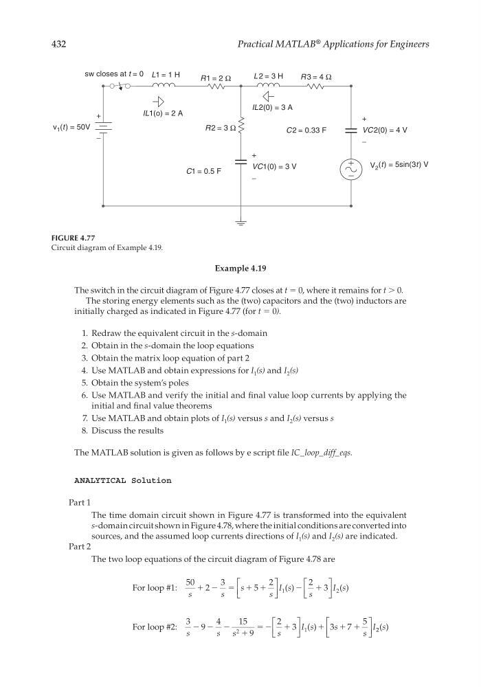
The switch in the circuit diagram of Figure 4.77 closes at t = 0, where it remains for t > 0.
The storing energy elements such as the (two) capacitors and the (two) inductors are
initially charged as indicated in Figure 4.77 (for t = 0).
1. Redraw the equivalent circuit in the s-domain
2. Obtain in the s-domain the loop equations
3. Obtain the matrix loop equation of part 2
4. Use MATLAB and obtain expressions for I 1 (s) and I 2 (s)
5. Obtain the system’s poles
6. Use MATLAB and verify the initial and fi nal value loop currents by applying the
initial and fi nal value theorems
7. Use MATLAB and obtain plots of I 1 (s) versus s and I 2 (s) versus s
8. Discuss the results
The MATLAB solution is given as follows by e script fi le IC_loop_diff_eqs.
ANALYTICAL Solution
Part 1
The time domain circuit shown in Figure 4.77 is transformed into the equivalent
s-domain circuit shown in Figure 4.78, where the initial conditions are converted into
sources, and the assumed loop currents directions of I 1 (s) and I 2 (s) are indicated.
Part 2
The two loop equations of the circuit diagram of Figure 4.78 are
For loop #1:
50 2
3
5
2
2 3
1
2
s
s
s
s
I s
s
I s
ϩ
ϭ ϩ ϩ
ϩ
Ϫ
Ϫ
( )
( )
For loop #2:
3 9
4
15
9
2 3
3
7
5
2
1
s
s s
s
I s
s
s
I
Ϫ Ϫ Ϫ
Ϫ
ϩ
ϭ
ϩ
ϩ
ϩ ϩ
( )
2 2 ( )
s
v 1 (t) = 50V
V 2
sw closes at t = 0 L1 = 1 H
L 2 = 3 H
R1 = 2 Ω
R 2 = 3 Ω
R 3 = 4 Ω
C1 = 0.5 F
C 2 = 0.33 F
IL1(o) = 2 A
IL2(0) = 3 A
+
VC1(0) = 3 V
−
+
VC 2(0) = 4 V
−
(t ) = 5sin(3t ) V
+
−
FIGURE 4.77
Circuit diagram of Example 4.19.
CRC_47760_CH004.indd 432
CRC_47760_CH004.indd 432
7/28/2008 12:26:19 PM
7/28/2008 12:26:19 PM
Practical MATLAB
® Applications for Engineers
Example 4.19
The switch in the circuit diagram of Figure 4.77 closes at t = 0, where it remains for t > 0.
The storing energy elements such as the (two) capacitors and the (two) inductors are
initially charged as indicated in Figure 4.77 (for t = 0).
1. Redraw the equivalent circuit in the s-domain
2. Obtain in the s-domain the loop equations
3. Obtain the matrix loop equation of part 2
4. Use MATLAB and obtain expressions for I 1 (s) and I 2 (s)
5. Obtain the system’s poles
6. Use MATLAB and verify the initial and fi nal value loop currents by applying the
initial and fi nal value theorems
7. Use MATLAB and obtain plots of I 1 (s) versus s and I 2 (s) versus s
8. Discuss the results
The MATLAB solution is given as follows by e script fi le IC_loop_diff_eqs.
ANALYTICAL Solution
Part 1
The time domain circuit shown in Figure 4.77 is transformed into the equivalent
s-domain circuit shown in Figure 4.78, where the initial conditions are converted into
sources, and the assumed loop currents directions of I 1 (s) and I 2 (s) are indicated.
Part 2
The two loop equations of the circuit diagram of Figure 4.78 are
For loop #1:
50 2
3
5
2
2 3
1
2
s
s
s
s
I s
s
I s
ϩ
ϭ ϩ ϩ
ϩ
Ϫ
Ϫ
( )
( )
For loop #2:
3 9
4
15
9
2 3
3
7
5
2
1
s
s s
s
I s
s
s
I
Ϫ Ϫ Ϫ
Ϫ
ϩ
ϭ
ϩ
ϩ
ϩ ϩ
( )
2 2 ( )
s
v 1 (t) = 50V
V 2
sw closes at t = 0 L1 = 1 H
L 2 = 3 H
R1 = 2 Ω
R 2 = 3 Ω
R 3 = 4 Ω
C1 = 0.5 F
C 2 = 0.33 F
IL1(o) = 2 A
IL2(0) = 3 A
+
VC1(0) = 3 V
−
+
VC 2(0) = 4 V
−
(t ) = 5sin(3t ) V
+
−
FIGURE 4.77
Circuit diagram of Example 4.19.
CRC_47760_CH004.indd 432
CRC_47760_CH004.indd 432
7/28/2008 12:26:19 PM
7/28/2008 12:26:19 PM