

428
Practical MATLAB
® Applications for Engineers
Example 4.18
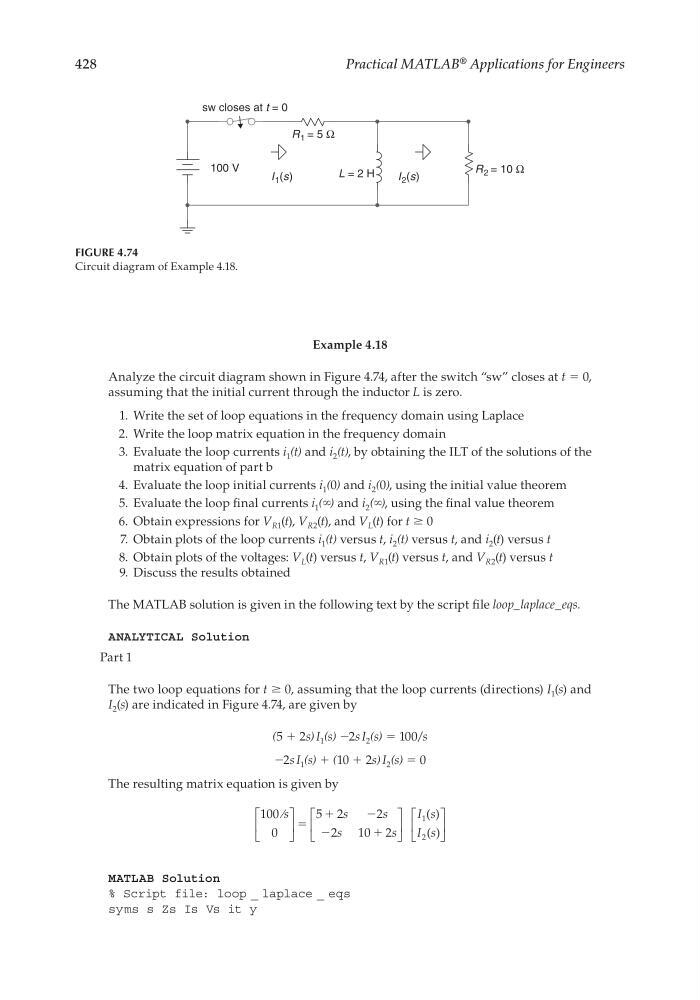
Analyze the circuit diagram shown in Figure 4.74, after the switch “sw” closes at t = 0,
assuming that the initial current through the inductor L is zero.
1. Write the set of loop equations in the frequency domain using Laplace
2. Write the loop matrix equation in the frequency domain
3. Evaluate the loop currents i 1 (t) and i 2 (t), by obtaining the ILT of the solutions of the
matrix equation of part b
4. Evaluate the loop initial currents i 1 (0) and i 2 (0), using the initial value theorem
5. Evaluate the loop fi nal currents i 1 (∞) and i 2 (∞), using the fi nal value theorem
6. Obtain expressions for V R1 (t), V R2 (t), and V L (t) for t ≥ 0
7. Obtain plots of the loop currents i 1 (t) versus t, i 2 (t) versus t, and i 2 (t) versus t
8. Obtain plots of the voltages: V L (t) versus t, V R1 (t) versus t, and V R2 (t) versus t
9. Discuss the results obtained
The MATLAB solution is given in the following text by the script fi le loop_laplace_eqs.
ANALYTICAL Solution
Part 1
The two loop equations for t ≥ 0, assuming that the loop currents (directions) I 1 (s) and
I 2 (s) are indicated in Figure 4.74, are given by
(5 + 2s) I 1 (s) −2s I 2 (s) = 100/s
−2s I 1 (s) + (10 + 2s) I 2 (s) = 0
The resulting matrix equation is given by
100
0
5 2
2
2
10 2
1
2
⁄s
s
s
s
s
I s
I s
ϭ
ϩ
Ϫ
ϩ
Ϫ
( )
( )
MATLAB Solution
% Script file: loop _ laplace _ eqs
syms s Zs Is Vs it y
100 V
sw closes at t = 0
R 1 = 5 Ω
R 2 = 10 Ω
L = 2 H
I 1 (s)
I 2 (s)
FIGURE 4.74
Circuit diagram of Example 4.18.
CRC_47760_CH004.indd 428
CRC_47760_CH004.indd 428
7/28/2008 12:26:18 PM
7/28/2008 12:26:18 PM
Practical MATLAB
® Applications for Engineers
Example 4.18
Analyze the circuit diagram shown in Figure 4.74, after the switch “sw” closes at t = 0,
assuming that the initial current through the inductor L is zero.
1. Write the set of loop equations in the frequency domain using Laplace
2. Write the loop matrix equation in the frequency domain
3. Evaluate the loop currents i 1 (t) and i 2 (t), by obtaining the ILT of the solutions of the
matrix equation of part b
4. Evaluate the loop initial currents i 1 (0) and i 2 (0), using the initial value theorem
5. Evaluate the loop fi nal currents i 1 (∞) and i 2 (∞), using the fi nal value theorem
6. Obtain expressions for V R1 (t), V R2 (t), and V L (t) for t ≥ 0
7. Obtain plots of the loop currents i 1 (t) versus t, i 2 (t) versus t, and i 2 (t) versus t
8. Obtain plots of the voltages: V L (t) versus t, V R1 (t) versus t, and V R2 (t) versus t
9. Discuss the results obtained
The MATLAB solution is given in the following text by the script fi le loop_laplace_eqs.
ANALYTICAL Solution
Part 1
The two loop equations for t ≥ 0, assuming that the loop currents (directions) I 1 (s) and
I 2 (s) are indicated in Figure 4.74, are given by
(5 + 2s) I 1 (s) −2s I 2 (s) = 100/s
−2s I 1 (s) + (10 + 2s) I 2 (s) = 0
The resulting matrix equation is given by
100
0
5 2
2
2
10 2
1
2
⁄s
s
s
s
s
I s
I s
ϭ
ϩ
Ϫ
ϩ
Ϫ
( )
( )
MATLAB Solution
% Script file: loop _ laplace _ eqs
syms s Zs Is Vs it y
100 V
sw closes at t = 0
R 1 = 5 Ω
R 2 = 10 Ω
L = 2 H
I 1 (s)
I 2 (s)
FIGURE 4.74
Circuit diagram of Example 4.18.
CRC_47760_CH004.indd 428
CRC_47760_CH004.indd 428
7/28/2008 12:26:18 PM
7/28/2008 12:26:18 PM