

Fourier and Laplace
401
F10 =10*sin(w*tau10/2)./(w*tau10/2);
subplot(3,1,1)
plot(w,F1);
ylabel(‘Amplitude’);
title(‘Spectrum of pulse with tau=1’);
axis([-10 10 -1 2]);
subplot(3,1,2);plot(w,F5);
ylabel(‘Amplitude’);
title(‘Spectrum of pulse with tau=5’);
axis([-7 8 -4 6]);
subplot(3,1,3);plot(w,F10);
xlabel(‘frequency w (in rad/sec)’);
ylabel(‘Amplitude’);
title(‘Spectrum of pulse with tau=10’);
axis([-10 10 -4 11]);
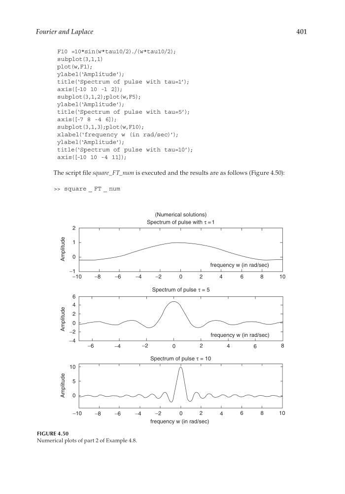
The script fi le square_FT_num is executed and the results are as follows (Figure 4.50):
>> square _ FT _ num
frequency w (in rad/sec)
frequency w (in rad/sec)
(Numerical solutions)
Spectrum of pulse with τ = 1
2
0
6
4
2
−2
−4
0
1
−1
−10
10
5
0
−8
−6
−6
−10
−8
−6
−4
−2
0
2
−4
−4
−2
−2
0
0
2
2
4
4
6
6
8
8
10
Spectrum of pulse τ = 5
Spectrum of pulse τ = 10
frequency w (in rad/sec)
4
6
8
10
Amplitude
Amplitude
Amplitude
FIGURE 4.50
Numerical plots of part 2 of Example 4.8.
CRC_47760_CH004.indd 401
CRC_47760_CH004.indd 401
7/28/2008 12:26:12 PM
7/28/2008 12:26:12 PM
401
F10 =10*sin(w*tau10/2)./(w*tau10/2);
subplot(3,1,1)
plot(w,F1);
ylabel(‘Amplitude’);
title(‘Spectrum of pulse with tau=1’);
axis([-10 10 -1 2]);
subplot(3,1,2);plot(w,F5);
ylabel(‘Amplitude’);
title(‘Spectrum of pulse with tau=5’);
axis([-7 8 -4 6]);
subplot(3,1,3);plot(w,F10);
xlabel(‘frequency w (in rad/sec)’);
ylabel(‘Amplitude’);
title(‘Spectrum of pulse with tau=10’);
axis([-10 10 -4 11]);
The script fi le square_FT_num is executed and the results are as follows (Figure 4.50):
>> square _ FT _ num
frequency w (in rad/sec)
frequency w (in rad/sec)
(Numerical solutions)
Spectrum of pulse with τ = 1
2
0
6
4
2
−2
−4
0
1
−1
−10
10
5
0
−8
−6
−6
−10
−8
−6
−4
−2
0
2
−4
−4
−2
−2
0
0
2
2
4
4
6
6
8
8
10
Spectrum of pulse τ = 5
Spectrum of pulse τ = 10
frequency w (in rad/sec)
4
6
8
10
Amplitude
Amplitude
Amplitude
FIGURE 4.50
Numerical plots of part 2 of Example 4.8.
CRC_47760_CH004.indd 401
CRC_47760_CH004.indd 401
7/28/2008 12:26:12 PM
7/28/2008 12:26:12 PM